A Reality Check on DeepSeek's Distributed File System Benchmarks
Series
- An Intro to DeepSeek’s Distributed File System
- A Reality Check on DeepSeek’s Distributed File System Benchmarks
- Network Storage and Scaling Characteristics of a Distributed Filesystem
How should we analyze 3FS?
In my previous post, I introduced DeepSeek’s 3FS distributed file system – exploring its architecture, components, and the CRAQ protocol that provides its consistency guarantees. Now, I want to take a closer look at the published benchmark results and performance claims.
When evaluating distributed systems, there’s a tendency to jump straight into complex profiling tools and detailed metrics.Trying out perf, strace for syscalls, iostat for disk, it’s essentially throwing random darts until you hit something However, I find tremendous value in performing an initial “performance reality check” on numbers and graphs. The check uses reference numbers from other sources, such as hardware manufacturer specifications or existing benchmarks, to provide a baseline quickly for a particular systemFor example, when I drive a car on the highway, I try to match the speed to the other cars around me. Without that reference, it might turn out that I’m over the speed limit if I’m not constantly checking the speed gauge. This approach helps identify potential bottlenecks or inconsistencies before deploying software tools for deeper investigation.
A “performance reality check” can reveal the following:
- It validates whether benchmark results match what we’d expect based on the hardware configuration
- It helps identify which components (network, storage, cpu, etc) represent the main bottleneck
- It reveals the percentage of theoretical capacity actually being utilized
- It verifies whether the authors’ claims are valid and how they may have arrived at those conclusions
To illustrate this method, imagine a startup making claims about their new database – “built for AI training” and “hyper performance”. They showcase a benchmark from a single node:

The system managed to read 250 GB in the total time, which seems impressive! However, this is like saying I drove 100 miles without mentioning whether it took an hour or 10. The rate (GB per second) reveals the actual work accomplished relative to time invested. Let’s approximate it by drawing a slope through the data.

2 GB/s. Great number, but one might wonder – what should we compare this number to?
A start might be to ask is if this utilizing the full potential of the hardware? Looking up modern SSD specifications for random reads and plotting that on the graph can reveal the following:

Theoretically, the system should reach 500 GB by the end of the test period!
The benchmark is only utilizing about half of the available device bandwidth. This might raise some eyebrows about their performance claims – where are the bottlenecks?
This analytical approach is exactly what I’ll apply to DeepSeek’s 3FS benchmarks throughout this post. By calculating what the hardware should deliver and comparing it to what 3FS actually achieves, we can identify where the possible bottlenecks lie and assess whether performance claims hold up.While not exact, these comparisons give us immediate insights that would take days to obtain through benchmarking
Into analyzing 3FS
I’ll be examining three different workloads that showcase 3FS in action:
- AI training jobs featuring a massive amount of reads
- GraySort, a synthetic sorting benchmark with a mix of reads and writes
- KV cache in operation, representing LLM inference workloads with random reads
Each benchmark consists of two main components – client and storage. The client sends a request to read/write to the storage node over a network. Then, the storage node reads/writes the data to its device(s) and responds to the client by sending a message back. Thus, the two main hardware components one should analyze closely are network and storage.
For each benchmark, I’ll break down the hardware configuration, calculate theoretical maximums, and analyze how close the system comes to achieving its potential performance. Through this analysis, we’ll develop intuition about 3FS’s real-world capabilities before even deploying it.
Let’s start by examining what could be 3FS’s most important benchmark: training throughput for AI workloads.
First workload: Training job
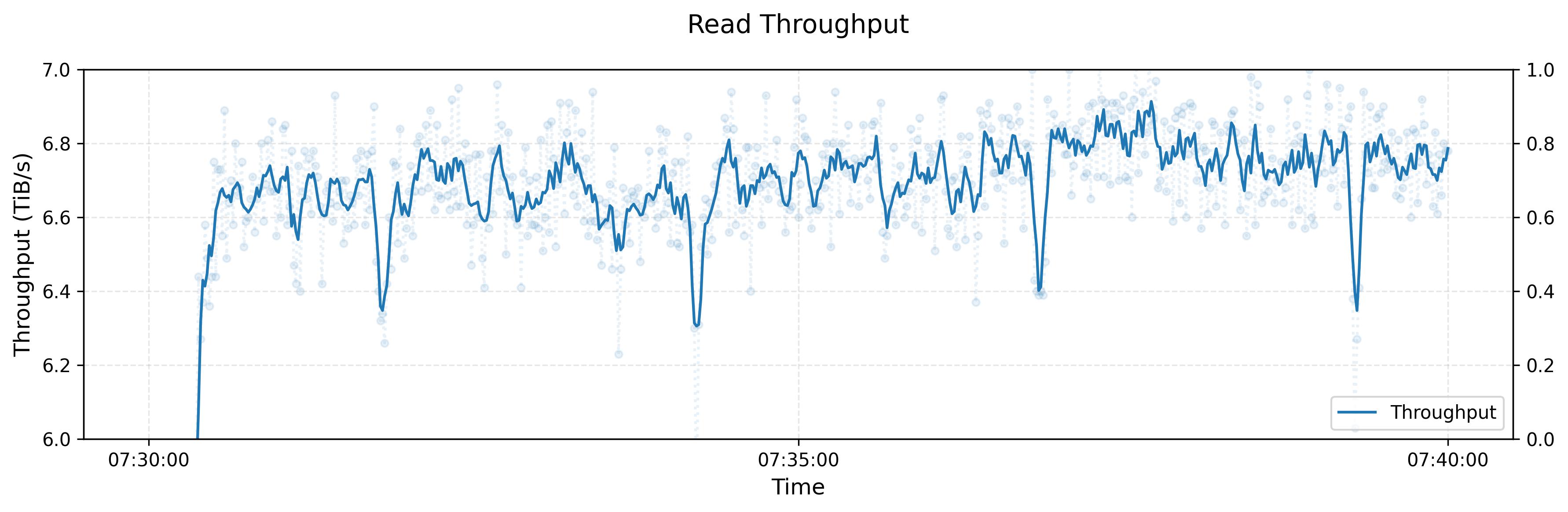
A training workload typically involves GPU nodes acting as clients that read data (text, images, etc.) from storage nodes to train deep neural networks like language or diffusion models. The throughput hovers around 6.6 TB/sIt’s not made explicit if this read throughput is the average or median. I would assume the average throughput. on average, with peak throughput reaching 8 TB/s as reported in the Fire-Flyer AI-HPC paper.
Here’s the hardware configuration the benchmark uses:
| Node Type | Component | Specification |
|---|---|---|
| Client | Number of nodes | 500 |
| Network | 1 × 200Gbps NIC | |
| Storage | Number of nodes | 180 |
| Disk | 16 × 14TB PCIe 4.0 NVMe SSDs | |
| Network | 2 × 200Gbps NICs | |
| Memory | 512 GB DDR4-3200MHz | |
| CPU | 2 × AMD 32 Cores EPYC Rome/Milan |
Let’s apply the “performance reality check” on these numbers – Below are some back-of-the-envelope calculationsBack-of-the-envelope calculations involve performing rough additions and multiplications to get an approximate number within the range of the actual value to get an idea of the theoretical limitsThe authors don’t list the SSD used in the benchmark, so I’ll be using a Micron 7450 15.36TB U.3 enterprise SSD as reference of the benchmark. Click the “Show calculations” toggle button in the top right to see the detailed breakdown. The base numbers (7GB/s, 4GB/s, 6GB/s, 2GB/s) come from reference SSD specifications I selected to represent this workload. Also, the NIC’s throughput is measured in Gbps instead of GB/s. Performing the conversion: 200Gbps ÷ 8 = 25GB/s.
| Node Type | Metric | Per Unit | Per Node | Entire Cluster |
|---|---|---|---|---|
| Storage (180) | Disk - Sequential Read | 7 GB/s | 112 GB/s | 20.16 TB/s |
| Disk - Random Read | 4 GB/s | 64 GB/s | 5.04 TB/s | |
| Disk - Sequential Write | 6 GB/s | 96 GB/s | 7.56 TB/s | |
| Disk - Random Write | 2 GB/s | 32 GB/s | 2.52 TB/s | |
| Network | 25 GB/s | 50 GB/s | 9 TB/s | |
| Client (500) | Network | 25 GB/s | 25 GB/s | 12.5 TB/s |
| ML Training | Avg Read Throughput | N/A | N/A | 6.6 TB/s |
| ML Training | Peak Read Throughput | N/A | N/A | 8 TB/s |
From these numbers, one can observe that:
- The client’s network will not be a bottleneck (12.5 TB/s client network throughput > 9 TB/s storage network throughput)Hover over the text to see the numbers highlighted in the table!
- The training job workload indicates a mix of sequential/random read because 6.6 TB/s average throughput is greater than the maximum disk random read throughput (6.6 TB/s > 5 TB/s)
- The storage nodes will be bottlenecked by network or disk depending on the type of workload. A network bottleneck occurs when the workload primarily consists of sequential readsAn example of this type of workload is reading a large file (movie, song, etc) in order to transfer the data to another device and the network cannot match the sequential throughput (20 TB/s > 9 TB/s)
- When workload primarily consist random reads, sequential write, or random writes, the storage becomes the bottleneck rather than the network. (5 TB/s, 7.5 TB/s, 2.5 TB/s < 9 TB/s)
- This workload is most likely bottlenecked by network bandwidth. The sequential read throughput can reach up to 20 TB/s and the network throughput is 9 TB/s, but the peak throughput of 8 TB/s and average throughput of 6.6 TB/s are below the network limit and well below the maximum sequential throughput.
Sometimes it’s hard to look at numbers. If we replot the numbers relative to the maximum sequential throughput of a SSD and lay the numbers on a bar plot, we can get a better idea of where the numbers are:

The visualization reveals some interesting insights about system utilization that we have already pointed out:
- The average 6.6 TB/s represents:
- 33% of theoretical sequential disk throughput (6.6 / 20 TB/s)
- 73% of available network bandwidth (6.6 / 9 TB/s)
- The peak 8 TB/s achieves:
- 40% of theoretical sequential disk throughput (8 / 20 TB/s)
- 88% of available network bandwidth (8 / 9 TB/s)
The data clearly shows that network bandwidth becomes the primary bottleneck. This suggests two potential optimization paths: either remove half of the SSDs from each storage node or upgrade to 800 Gbps NICs to unlock full sequential read potential. However, implementing these changes presents practical challenges. Hardware platforms often have limitations that prevent NIC upgrades and removing storage may leave PCIe slots unused. And, pure cost alone may make changing the existing setup unreasonable.
Also, why does peak throughput cap at 8 TB/s rather than closer to the theoretical network limit of 9 TB/s? Is this a fundamental software limitation, or does it reflect overhead associated with network operationsCould be TCP or RDMA overhead at this scale?I’ll have better answers to such questions when I run benchmarks on 3FS
Revisiting the training job with some background
Now, let’s revisit the throughput over time graph with these background numbers in mind.
The graph shows read throughput hovering around 6.6 TB/s, which represents approximately 73% of the theoretical 9 TB/s network capacityI typically set 0 as the starting point for the y axis, which gives you an absolute base number that you can compare to. This leaves 27% of potential throughput unutilized, suggesting possible system bottlenecks such as:
- Metadata communication network overhead (think TCP headers)
- Network completion delays before reading
- Workload imbalance creating hot nodes
- FUSE bottlenecks in the client for file operations
- Kernel overhead in managing communication and disk I/O
- Straggler storage nodes slowed by disk issues (temperature, wear)
- Native filesystem (XFS, ext4) overheads
- …
Dips in the training job
The periodic dips in throughput are somewhat interesting:

These dips could originate from either the filesystem or the workload itself. The filesystem might have internal mechanisms (periodic flushing, lock contention, etc.) that could cause these performance drops. But, because the dips occur at regular ~2.5 second intervals, it strongly suggests that checkpointing operations might cause these dropsThe dips hover around 6.3 TB/s, so at 6.6 TB/s average, that’s a 4.5% drop in throughput (300 GB/s / 6600 GB/s). These dips last roughly 10% of the time between peak points, so overall throughput may decrease by about 0.45% - not particularly significant. as the parts of the model may need to pause training while checkpoint data is written.
Next up: Gray Sort Benchmark
What is Gray Sort?
Gray Sort is a synthetic benchmark that tests how quickly a system can sort largeLarge as in terabytes large, and definitely will not fit on a single machine amounts of data. The workload follows a specific pattern that stresses both sequential and random I/O operations:
- Read unsorted data from storage into memory (sequential reads)
- Sort each data chunk in memory
- Write the sorted chunks back to storage (random-ish writes)
- Read the fetching other node’s sorted chunks and merge them in memory (random-ish reads)
- Write the merged results back to disk (random-ish writes)
- Repeat until all data is fully sorted
- Write the full sorted result to disk (sequential writes)
This alternating pattern of reads and writes, combined with both sort and merge phases, makes it a standard test for distributed filesystem performanceSounds like a MapReduce workload, essentially aggregating in keys in a range to a partition and then performing some operation on that range (merging in this case).
Initial Look at the Graphs
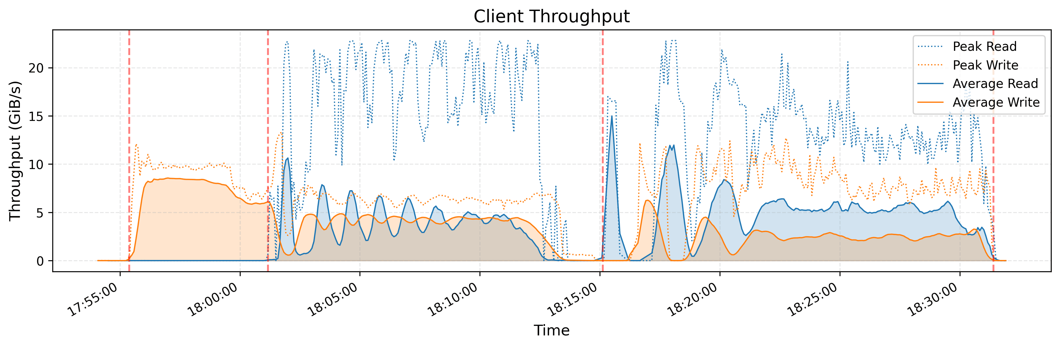
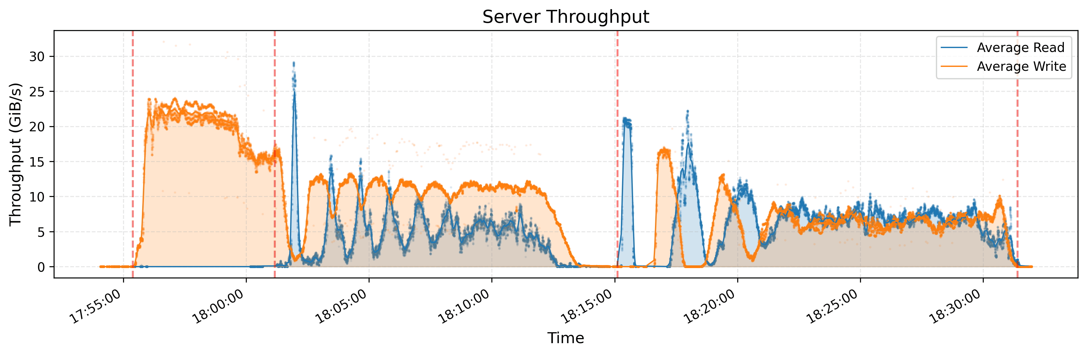
Note that orange represents writes and blue represents reads.
Looking at the orange dotted lines separating the algorithm phases, there’s a clear pattern. The phase before the first dotted line is pure writes – the system writing the unsorted data to the storage. After that, we see mixed read/write workloads that gradually shift toward being more read-heavy as the sorting progressesAs more and more sorted runs get merged together, there are fewer write operations needed since each merge pass consolidates multiple inputs into fewer outputs, while the read operations increase to fetch data from the remaining sorted runs. This pattern is observable when comparing workload differences between the 18:05:00-18:10:00 and 18:25:00-18:30:00 time ranges in the server throughput graph.
A few observations jump out:
- If one were to eyeball the average combined (read / write) throughput per phase, it would hover around ~10-15 GB/s.
- Clients peak at around 10 GB/s for writes while peaking 22 GB/s for reads.
- Storage nodes peak at 22 GB/s for writes and 30 GB/s for reads – their throughput is approximately twice the amount of the client’s average throughput, which makes sense given there are twice as many clients as storage nodes. We see this listed in the next section on hardware configuration.
Hardware Configuration
For this benchmark, 3FS was deployed with the following hardware setup:
| Node Type | Component | Specification |
|---|---|---|
| Client | Number of nodes | 50 |
| Network | 1 × 200Gbps NIC | |
| Memory | 2.2TB DDR4 | |
| Storage | Number of nodes | 25 |
| Disk | 16 × 14TB PCIe 4.0 NVMe SSDs | |
| Network | 2 × 400Gbps NICs | |
Analysis
The main difference from the previous benchmark is that there are twice as many clients as there are storage nodes (compared to 3x from previous benchmark) and the storage nodes have twice as much network bandwidth!
Let’s calculate the theoretical performance limits for this configuration:
| Node Type | Metric | Per Unit | Per Node | Entire Cluster |
|---|---|---|---|---|
| Storage (25) | Disk - Sequential Read | 7 GB/s | 112 GB/s | 2.8 TB/s |
| Disk - Random Read | 4 GB/s | 64 GB/s | 1.6 TB/s | |
| Disk - Sequential Write | 6 GB/s | 96 GB/s | 2.4 TB/s | |
| Disk - Random Write | 2 GB/s | 32 GB/s | 0.8 TB/s | |
| Network | 100 GB/s | 100 GB/s | 2.5 TB/s | |
| Client (50) | Network | 25 GB/s | 25 GB/s | 1.25 TB/s |
| Gray Sort | Client Write Peak | N/A | ~10 GB/s | N/A |
| Gray Sort | Client Read Peak | N/A | ~22 GB/s | N/A |
| Gray Sort | Server Write Peak | N/A | ~22 GB/s | N/A |
| Gray Sort | Server Read Peak | N/A | ~30 GB/s | N/A |
The performance numbers reveal an interesting pattern. In the first phase, the server write peak achieves ~22 GB/s out of 32 GB/s random write capacity (69% utilization). In the second phase, the server read peak reaches ~30 GB/s out of 64 GB/s random read capacity (47% utilization), which is quite a bit lower than the relative utilization for writes. However, comparing to sequential read throughput ~30 GB/s vs 112 GB/s (27% utilization) strongly signals that the workload is predominantly random rather than sequential.
Let’s take a look at the numbers:
- Storage nodes peak at 22 GB/s writes and 30 GB/s reads, well below the 100 GB/s network capacity
- Client read peak achieves 88% of network capacity (22 GB/s out of 25 GB/s)
- Client write peak hits only 40% of network capacity (10 GB/s out of 25 GB/s)Why does the writes not peak nearly as high as reads? A reason might be from CRAQ’s consistency guarantees - each write must traverse the entire chain (head → middle → tail → back), which makes performance predictable unlike reads. Reads can come from the follower, or cause a consistency check at the tail
The bottleneck here is clearly the number of clients. With the storage nodes far from saturated, we could support more clients. How many? If we want to saturate the storage sequential write capacity of 2.4 TB/s and each client can push 25 GB/s:
2.4 TB/s ÷ 25 GB/s = ~96 clients
Nearly double the current 50 clients! This suggests the current configuration may be significantly underutilizing the storage infrastructure.
Interestingly, the storage write peak (22 GB/s) slightly exceeds client write peak (20 = 2 × 10 GB/s). With 50 clients at 10 GB/s distributed across 25 storage nodes, each node should see ~20 GB/s, with the extra 2 GB/s coming somewhere – maybe, from CRAQ protocol overhead?CRAQ requires writes to propagate through chains, potentially creating additional write traffic beyond what clients generate
The end-to-end performance measurements, however, reveal an unexpected pattern: the benchmark notes mention achieving 3.66 TB/min – 61 GB/s aggregate throughput, which doesn’t sound too bad. But that’s just 4.88% of the 1.25 TB/s client network capacity. This suggests that most of bottleneck might not be network or disk at all – it could be even be CPU/memory bound from the sorting computation itself.
Caching the key-value pairs of the transformer
What is the KV Cache?
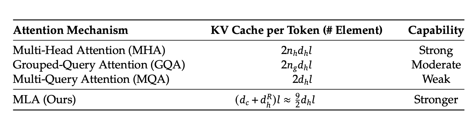
The KV cache stores the key-value pairs from attention mechanisms during LLM inference. Instead of recomputing these values for every new token, the system caches them to dramatically reduce computational overhead by trading computation for storage. For models like DeepSeek’s R1, this cache becomes substantial – each token requires approximately 70KB of storage in FP16 format.
This workload represents an important real-world use case for 3FS. As LLMs process longer contexts and serve more users concurrently, the storage system must handle both massive reads (loading cached values) and periodic deletions (garbage collecting expired entries).
Initial Look at the Graphs

The graphs show per-client performance for KV cache operations. Looking at the read throughput graph:
- Average throughput hovers around 3 GB/s
- Peak throughput reaches approximately 40 GB/s
- Which is more than 13x difference between average and peak
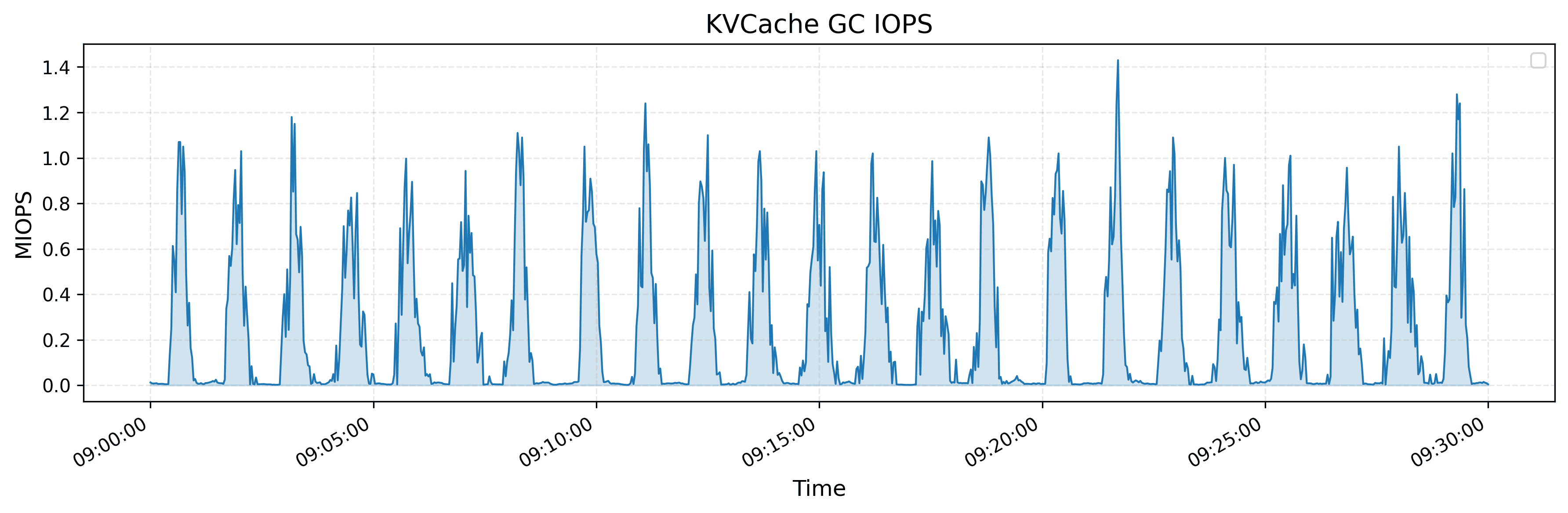
The GC IOPS graph reveals:
- Periodic bursts of deletion operations reaching 1-1.4M IOPS
- ~4 bursts per 5-minute interval
- Lasts around ~40 seconds each, followed by similar periods of low activity
Unfortunately, the authors don’t specify the complete hardware configuration - we only know each client has a 400 Gbps NIC (50 GB/s). This means the peak 40 GB/s achieves 80% network utilization, while average performance uses only 6% of available bandwidth.
Analyzing the Workload
The read pattern is fundamentally random – individual KV entries are scattered across storage. However, each 70KB entry spans multiple 4KB blocksSSDs read data in fixed-size blocks, typically 4KB. A 70KB entry requires reading 18 consecutive blocks, resulting in sequential device-level reads despite the random access pattern per entry.
Let me calculate what these throughput numbers mean for token processing:
Expand for calculations for KV cache entry
{
    "vocab_size": 129280,
    "dim": 7168,
    "inter_dim": 18432,
    "moe_inter_dim": 2048,
    "n_layers": 61,
    "n_dense_layers": 3,
    "n_heads": 128,
    "n_routed_experts": 256,
    "n_shared_experts": 1,
    "n_activated_experts": 8,
    "n_expert_groups": 8,
    "n_limited_groups": 4,
    "route_scale": 2.5,
    "score_func": "sigmoid",
    "q_lora_rank": 1536,
    "kv_lora_rank": 512,
    "qk_nope_head_dim": 128,
    "qk_rope_head_dim": 64,
    "v_head_dim": 128,
    "dtype": "fp8"
}
Given:
- kv_lora_rank = 512
- qk_rope_head_dim = 64
- n_layers = 61
Per token: (512 + 64) × 61 = 35,136 elements
In FP16 format (2 bytes per element) = 70,272 bytes ≈ 70KB per token In FP8 format (1 byte per element) = 35,136 bytes ≈ 35KB per token
With 70KB per token:
- Average throughput (3 GB/s) processes ~43,000 tokens/second per client
- Peak throughput (40 GB/s) processes ~570,000 tokens/second per client
Given R1’s 128K context length:
- Average: Can read entire context in 3 seconds (128K ÷ 43K)
- Peak: Can read entire context in 0.22 seconds (128K ÷ 570K)
These numbers are impressive, but without knowing the number of concurrent users or typical context lengths, it’s hard to judge real-world performance.
Alignment Concerns
Here’s an issue the authors don’t address: alignment waste. Modern NVMe SSDs use 4KB block sizes, but KV cache entries are 70KB – not cleanly divisible.
Blocks needed = ⌈70,272 ÷ 4,096⌉ = 18 blocks
Actual storage = 18 × 4,096 = 73,728 bytes
Wasted space = 3,456 bytes (4.69%)
This 4.69% waste might seem small, but at scale it adds up. With enterprise SSDs costing ~$2,200 each:
- Cost per SSD: $103
- Cost per node (16 SSDs): ~$1,650
- Cost per 180 nodes: ~$297,000
- Cost per 10,000 nodes: ~$16,500,000
For a company running thousands of clusters, this alignment inefficiency could waste millions in storage costs.
Garbage Collection
The GC algorithm isn’t detailed, but entries likely get marked for deletion when no longer referenced. The deletion mechanism remains unclear - could involve bit flags, pointer updates, zeroing entries, or tombstone markers.
The periodic burst pattern (1-1.4M IOPS) suggests that it’s probably more efficient to threshold-based eviction or batch processing rather than continuous cleanup for this type of workload. While throughput remains stable during GC, these spikes could impact performance if disks are already near throughput capacityGarbage collection problems have appeared numerous times in many existing systems – showing up as compaction issues in RocksDB or auto vacuum spikes in Postgres.
Remaining feedback
Some critical information is absent from this benchmark, most notably the lack of latency graphs. For LLM serving, latency matters as much as throughput - users need consistent time-to-first-token and smooth text generation, or they’ll switch to another service (chatgpt, gemini, claude, etc…).
Someone at Deepseek clearly knows how to configure systems well if this is a real sample from a live system. The 80% peak utilization indicates a well-configured system with just enough headroom.Nobody wants that 3am call to discuss needing to setup more machines to handle the traffic
Closing Thoughts
The benchmarks focus exclusively on throughput, omitting latency metrics entirely. Not sure why they skipped latency – perhaps cost considerations took priority. While latency optimization is notoriously difficultStuart Cheshire: “It’s the latency, stupid”Jeff Dean on tail latencies at scale, my future evaluations will include latency measurements and explore optimizations to improve the latency.
Despite these limitations and critiques, the benchmarks align well with theoretical calculations and provide valuable insights into 3FS performance at scale.
In upcoming posts, I’ll benchmark 3FS myself to verify these graph/claims and dig deeper:
- Testing actual hardware limits vs theoretical calculations
- Measuring latency distributions, not just throughput
- Creating custom visualizations for storage and network performance patterns
- Validating if our back-of-the-envelope math holds up
- Profiling with various tools (perf, sampling, adapting source code) to identify bottlenecks
Acknowledgments
Thanks to Stefanos Baziotis, Ahan Gupta, and Vimarsh Sathia for reviewing this post.
Citation
To cite this article:
@article{zhu20253fs2,
  title = {A Reality Check on DeepSeek's Distributed File System Benchmarks},
  author = {Zhu, Henry},
  journal = {maknee.github.io},
  year = {2025},
  month = {June},
  url = "https://maknee.github.io/blog/2025/3FS-Performance-Journal-2/"
}
Enjoy Reading This Article?
Here are some more articles you might like to read next: