Network Storage and Scaling Characteristics of a Distributed Filesystem
Series
- An Intro to DeepSeek’s Distributed File System
- A Reality Check on DeepSeek’s Distributed File System Benchmarks
- Network Storage and Scaling Characteristics of a Distributed Filesystem
Table of Contents
- The Benchmarking Pyramid
- Network Baseline Benchmark
- Storage Baseline Benchmark
- 3FS Performance Analysis
- Wrapping up
Refresher
In my first post, I introduced DeepSeek’s 3FS distributed file system and performed a reality check in the second post. Now it’s time to see how 3FS performs in practice.
The Benchmarking Pyramid
Before diving into results, let’s talk about the understanding software performance from a high level. If we imagine performance understanding as an onion, peeling off each layer onion reveals deeper insightsEach layer gives us a deeper understanding. Without starting at the top, the discovering insights may be difficult

We started with napkin math in the first post, performed reality checks in the second, and now we’re ready for the next layer: microbenchmarking.
Why Microbenchmark?
Think of microbenchmarking as testing individual components in isolation. Instead of running a complex workload that does everything at once, we test one specific operation repeatedly until we understand its exact performance characteristics. It’s like measuring only how fast a car accelerates in a straight line instead of timing a trip through city traffic where you can’t tell if slowdowns are from stop signs, traffic lights, or congested highways.
But one might ask: why not jump straight to real workloads? Real workloads are messy. They mix reads, writes, different block sizes, and various access patterns. When something’s slow, is it the network? The disk? The software? That’s the challenge with macrobenchmarks and production workloads (the bottom layers of our pyramid). There’s too many variables at once. Microbenchmarks let us isolate each component and understand exactly where time is spentThey answer specific questions like: What’s the maximum throughput for sequential reads? How does latency change with queue depth? Where exactly does performance cliff when we increase parallelism?.
These benchmarks build intuition at multiple levels: from raw hardware performance to how exactly 3FS performs. Once one recognize these patterns, one can have intuition on related applications may be slow and how to fix itThis knowledge transfers across systems too – similar hardware will have similar characteristics regardless of the software running on top, and similar types of software (like filesystems) perform comparable operations.
In my previous posts, I made several predictions about 3FS performance based on napkin math and reality checks. Now that I have actual microbenchmark data, I can see how accurate those predictions were or how terribly off I was.
What we’re measuring and why
In this post, we’ll answer five key questions:
- What are the hardware limits? – Local SSD and InfiniBand benchmarks establish our ceiling
- How does 3FS compare? – Performance differences from local benchmarks and why they occur
- Is 3FS hardware-specific? – Does it require high-end hardware or work well on commodity clusters?DeepSeek’s paper describes a cluster with NVMe SSDs and 200Gb/s InfiniBand. What happens with SATA SSDs and 25Gb/s networking?
- How does 3FS scale? – Performance across different node counts and configurations
- What knobs matter? – Impact of block sizes, I/O patterns, and tuning parameters
This will start to build our intuition for how 3FS performs. The post includes many interactive graphs to explore the data yourselfI’ll highlight the interesting patterns so you don’t drown in numbers, sometimes benchmarks reveal surprising behaviors.
Single Node Benchmarking
Before diving into 3FS performance, we need to understand how our clusters performs. This section establishes baseline performance for both network and storage using standard tools.
Testing Environment
I have two contrasting setups that tell an interesting story:
| Component | Older Cluster (18 Nodes) | Modern Cluster (5 Nodes) |
|---|---|---|
| Node Count | 18 | 5 |
| Use case | Budget cluster | High-performance cluster |
| CPU | 10-core Intel E5-2640v4 (2017 era) | 2×36-core Intel Xeon Platinum (2021 era) |
| Memory | 64GB DDR4-2400 | 256GB DDR4-3200 |
| Storage | SATA SSD (480GB) | NVMe SSD (1.6TB PCIe 4.0) |
| Network | 25 Gbps (3.25 GB/s) | 100 Gbps (12.5 GB/s) |
The older cluster represents deployments using previous-generation hardware. The modern cluster represents somewhat current high-performance deployments. Comparing these reveals how 3FS performs across different hardware generationsI don’t have access to a high-end cluster with many NVMe drives and newer NICs. I’d love to have the setup that the 3FS team uses, but I’m just a student without access to those types of clusters 😔. I’ll be referring these clusters as old cluster and new cluster.
Expand to see more detailed hardware specifications
| Component | Older Cluster (18 Node Setup) | Modern Cluster (5 Node Setup) |
|---|---|---|
| Node Count | 18 | 5 |
| CPU | Ten-core Intel E5-2640v4 at 2.4 GHz | Two 36-core Intel Xeon Platinum 8360Y at 2.4GHz |
| RAM | 64GB ECC Memory (4x 16 GB DDR4-2400 DIMMs) | 256GB ECC Memory (16x 16 GB 3200MHz DDR4) |
| Disk | Intel DC S3520 480 GB 6G SATA SSD (OS & Workload) | Samsung 480GB SATA SSD (OS) Dell NVMe 1.6TB NVMe SSD (PCIe v4.0) (Workload) |
| Network | Mellanox ConnectX-4 25 GB NIC (1.25 GB/s, only one physical port at 25 Gbps) | Dual-port Mellanox ConnectX-6 100 Gb NIC (12.5 GB/s, Only one physical port enabled) |
Layout of Older Cluster:

Layout of Modern Cluster:

Network Baseline Benchmark
Distributed filesystems are only as fast as their network, which often becomes the primary bottleneck depending on the workload, as shown in my measurements in the previous post.
Since 3FS uses InfiniBand for data transfer, we first measure raw network performance using the ib_send, ib_read and ib_write benchmarks. These tests show us two things: how close we can get to the theoretical 12.5 GB/s (100 Gbps) limit, and how latency changes with different message sizesI will be profiling actual 3FS network traffic to observe what message sizes are used and how they map to these latency measurements in a later post.
The graph plots three key variables:
- Message Size (Z-axis): On a logarithmic scale, showing packet sizes from bytes to 10 megabytes
- Throughput (Y-axis): Data transfer rate in GB/s, with color mapping from blue (low) to red (high)
- Latency (X-axis): Transfer completion time in microseconds
Expand for instructions on how to interact with the graph
The results of the ib_read_bw benchmark are plotted in the interactive 3D graph below. You can click and drag to rotate the graph, and hovering over any data point will display its precise values.
The Test Type menu allows you to switch between different benchmark results (ib_write and ib_send). The View Mode can be changed to 2D, which helps observe latency variations more clearly.
IB benchmark unidirectional
IB Benchmark on unidirectional throughput/latency
Key observations from the throughput graph:
- All three operations (read, write, send) peak at ~11.5 GB/s (92% of theoretical) at 4K-8K message sizesSurprisingly, the send operation (two-sided) achieves the same bandwidth as one-sided RDMA operations. This is unexpected given the additional coordination overhead
- To achieve meaningful throughput (>10 GB/s), you need at least 4KB messages
Switching to the latency graph (Read Bandwidth -> Read Latency) reveals additional insights:
- At the same 4K message sizes, latency drops significantly to ~5μs when operating at ~1 GB/sThere’s some queuing going on? I’m not sure for this reason
Switching to 2D version of latency graph (Read Bandwidth -> Read Latency, 3D Graph -> 2D Graph):
- Two distinct latency regions emerge: a gentle increase from 5μs to 10μs (2 bytes to 64KB), then an almost linear scale beyond 64KBsThis is also true when we take a look at when the NIC is at full throughput. This makes the performance very predictable, which makes understanding network bottlenecks easier
- Latency variance remains stable across most message sizes (p50, p90, p99 are tightly grouped)
Since NICs support bidirectional communication, we also need to measure performance when traffic flows in both directions simultaneously:
IB benchmark bidirectional
IB Benchmark on bidirectional throughput/latency
The bidirectional results show similarities!
- At 4K-8K message sizes, we achieve double the throughput while latency drops from 30-60μs to 15-30μsThis counterintuitive result likely occurs because each direction gets dedicated hardware resources, allowing better pipeline utilization
- Combined bandwidth reaches ~23 GB/s (~92% of theoretical 25 GB/s)
- Latencies remain consistent with unidirectional measurements
These measurements give us concrete expectations for 3FS operations. For example, when 3FS performs a 3-node write (1KB from 3 storage nodes), the network alone will consume 3-10μs. Any latency above this represents other software/hardware overhead – chunk management, thread contention, or disk I/O.
Comparison to NCCL all_reduce_perf (for fun)
NCCL is the standard framework for GPU-to-GPU communication in machine learning clusters. Since GPUs also use InfiniBand for inter-node communication, I wanted to see if the same performance patterns emerge.
This test uses a 2-node cluster with 8x400Gbps InfiniBand NICs (~400GB/s total), typical for modern GPU clusters like 8xH100 setups.
NCCL all_reduce_perf
all_reduce_perf
The bandwidth pattern is similar (slow climb then rapid rise), but peak performance hits at ~512MB messages instead of 8KBLikely due to multiple NICs and the collective communication overhead of all_reduce operations. At the same 8KB message size where our InfiniBand tests peaked, NCCL only achieves ~0.24 GB/s @ ~20us.
Storage Baseline Benchmark
FIO is the standard tool for storage benchmarking on Linux, so I’ll be using that in the next section. As a heads up, the 3FS authors conveniently provide a custom FIO engine specifically for benchmarking their filesystemThis wasn’t in the original release – they added it after I started this analysis and I would have spent quie a bit of time writing it which we can compare to!
Local Storage Performance
Before measuring 3FS, we need baseline numbers for our SSDs. The following benchmarks show how bandwidth and latency change as we vary two key parameters:
- I/O depth: How many operations we submit before waiting for completion (think of it as the queue length)
- Job count: How many parallel processes are hammering the storage simultaneously
These SSD numbers will become our reference pointFor example, with a replication factor of 3, we might see 3x higher read throughput or 3x higher write latency, but this might not be the case! – when 3FS shows higher latency or lower throughput, we can quantify exactly how much overhead the distributed layer adds.
I’ll be benchmarking local ssd with io_uring, then 3fs with io_uring and then 3fs with its own custom iouring interface
I configured 3FS with a replication factor of 3.
Hardware Vendor Specifications
Before examining our benchmark results, let’s establish the theoretical performance limits according to hardware vendor specifications. These numbers represent the maximum performance we could theoretically achieve under ideal conditions:
| Performance Metric | Random Read | Sequential Read | Random Write | Sequential Write |
|---|---|---|---|---|
| SATA SSD | 276 MB/s | 450 MB/s | 380 MB/s | 72 MB/s |
| NVMe | 3.77 GB/s | 6.2 GB/s | 0.4 GB/s | 2.3 GB/s |
These theoretical limits come from the Intel DC S3520 SATA and Dell Enterprise NVMe specification sheets. In practice, our benchmarks will likely fall short of these numbers due to filesystem overhead, driver limitations, and real-world I/O patterns.
Also, the dramatic performance difference between SATA and NVMe storage is pretty immediate. NVMe provides roughly 10-15x higher throughput for most operations and this difference may impact how 3FS performs.
Benchmarking for Older Cluster
Local FIO results
Expand for instructions on how to interact with the graph
Controls:
- Test Type menu: Switch between Random Read, Sequential Read, Random Write, and Sequential Write
- Metric menu: Change between Bandwidth, IOPS, and various Latency measurements
3D Navigation:
- Click and drag: Rotate the view
- Scroll wheel: Zoom in/out
- Hover: See exact values for any data point
- Double-click: Reset to default view
Axes:
- X-axis: IO Depth (1 to 128)
- Y-axis: Number of Jobs (1 to 128)
- Color: The selected metric value (blue = low, red = high)
Scaling block size for local SSD
The first benchmark uses the older cluster to establish our local SSD baseline. I’m testing how performance changes with different block sizes (4K, 64K, 1MB, 4MB) to understand the storage characteristics of a SATA SSD. The local ssd was configured with xfs filesystem.
This is a lot of data. Feel free to jump between the interactive graphs and the performance analysis to explore the patterns.
4K Block Size - SSD XFS with IO_URING (Older)
Latency Percentiles
Small block (4K) performance using SSD with XFS filesystem and IO_URING driver on older cluster.
64k Block Size - SSD XFS with IO_URING (Older)
Latency Percentiles
Small block (64k) performance using SSD with XFS filesystem and IO_URING driver on older cluster.
1M Block Size - SSD XFS with IO_URING (Older)
Latency Percentiles
Performance characteristics of SSD with XFS filesystem using IO_URING driver with 1M block size on older cluster.
4m Block Size - SSD XFS with IO_URING (Older)
Latency Percentiles
Performance characteristics of SSD with XFS filesystem using IO_URING driver with 4m block size on older cluster.
Storage Performance Analysis for Local SSD
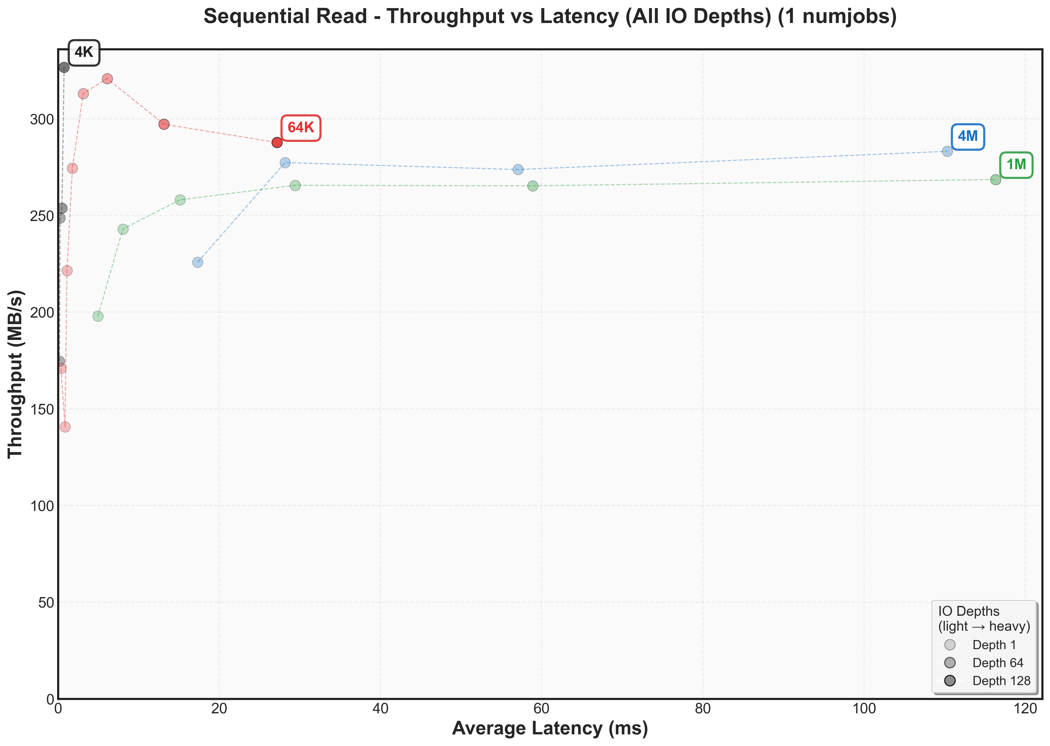
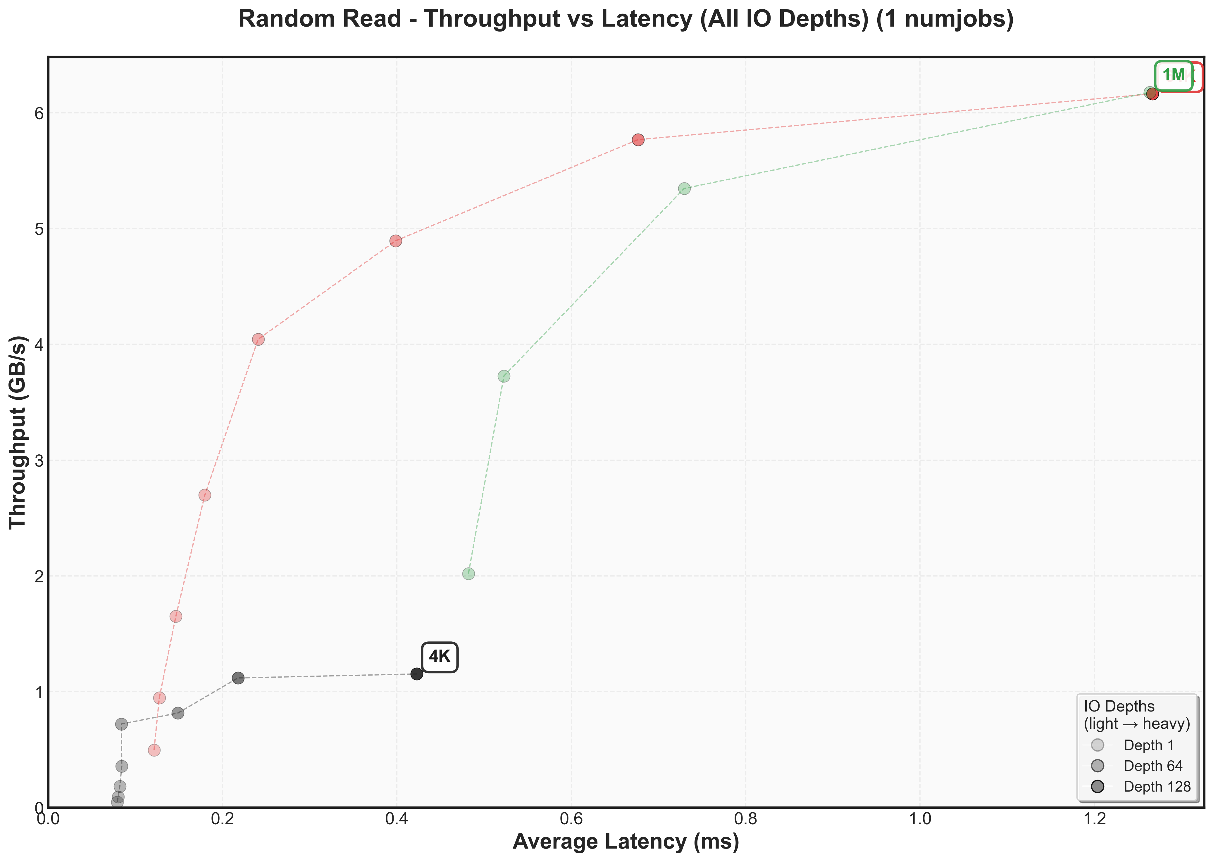
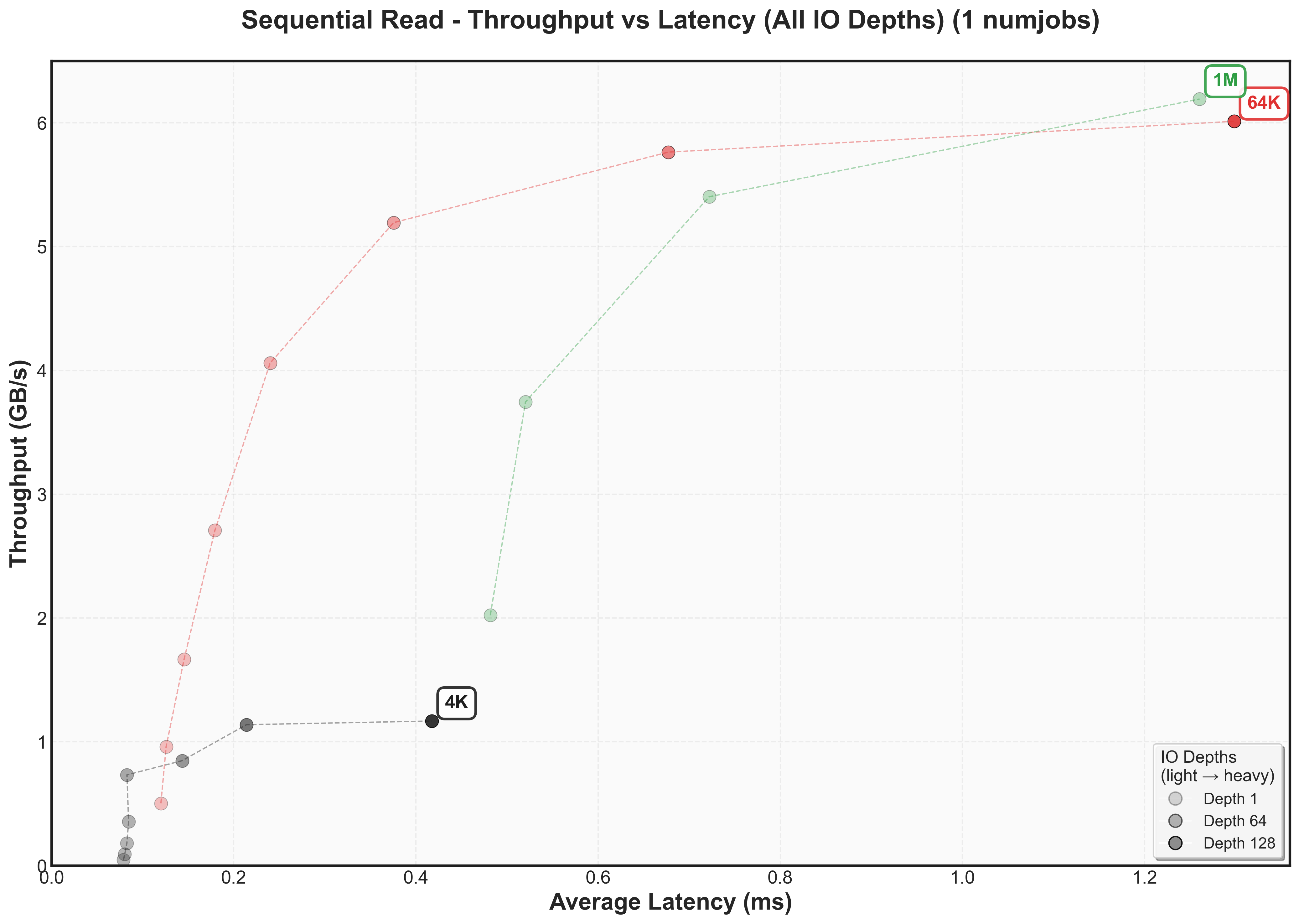
Let’s examine how performance changes across different block sizes by looking at a specific configuration point: various IO depths at 1 jobWhy 1 job? This removes one variable from our analysis, allowing us to focus on how IO depth affects performance. We’ll explore job scaling separately.

This graph reveals the classic throughput versus latency tradeoff for our SATA SSDThese plots are fundamental to understanding storage performance - they show exactly when a system hits diminishing returns. The Y-axis shows throughput (higher is better), while the X-axis shows latency (lower is better). Each colored line represents a different block size, with dots marking increasing IO depths.
First, let’s examine each axis independently:
- Y-axis (Throughput): 64K block sizes achieve the highest peak at 400 MB/s, while other sizes fall short: 4K reaches 250 MB/s, 1M hits 325 MB/s, and 4M peaks at 350 MB/s
- X-axis (Latency): Large block sizes (1M and 4M) show dramatically higher latency (80ms+) compared to smaller blocks size (4K and 64K)
The cool thing about throughput versus latency graphs is that there’s a knee point – where throughput stops increasing but latency continues climbingCertain systems even decrease throughput after this point as they may need to do additional work to manage work items. For 64K blocks, this occurs around IO depth 16-32, where we achieve ~400 MB/s at < 10ms.

Expand to view throughput versus latency graphs for other workloads
Expand to view throughput versus latency graphs scaling num jobs for random reads
These measurements reveal something frustrating, but also quite interesting: there’s no universal sweet spot. What works best depends entirely on whether you care more about latency or throughput and then that depends on what your workload looks like.
Couple of interesting things to observe:
- Latency increases in different amounts as block sizes increase
- Latency doubles as numjobs increases
- There’s not one block size that’s optimal for bandwidth for a workload. For random reads, it’s 64k. For sequential reads, it’s 4k.
- For lowest latency, use smaller block size, but the SSD most likely won’t fully saturate its bandwidth.
- Writes have different knee points than reads (for example, 4k sequential writes knee point caps at 150 MB/s while 4k sequential reads cap at 300 MB/s)
With these patterns established, let’s examine the NVMe fio benchmarks to see whether these observations hold true or if new patterns emerge.
Double checking if libaio has any difference
The performance shown in the graphs above represent io_uring. Are there any differences with another async io library (libaio?)
| Workload | Configuration | Bandwidth (MB/s) | Avg Latency (ms) | P99 Latency (ms) |
|---|---|---|---|---|
| Random Read | 4K iouring | 242.6 | 2.01 | 3.29 |
| Random Read | 1M iouring | 329.8 | 377.50 | 484.44 |
| Random Read | 4K libaio | 240.7 | 2.02 | 3.32 |
| Random Read | 1M libaio | 329.9 | 378.01 | 488.64 |
| Random Write | 4K iouring | 153.6 | 3.18 | 5.47 |
| Random Write | 1M iouring | 159.6 | 780.23 | 977.27 |
| Random Write | 4K libaio | 151.3 | 3.23 | 5.55 |
| Random Write | 1M libaio | 153.3 | 855.61 | 935.33 |
| Sequential Read | 4K iouring | 410.7 | 1.22 | 1.97 |
| Sequential Read | 1M iouring | 276.7 | 460.66 | 488.64 |
| Sequential Read | 4K libaio | 402.1 | 1.22 | 2.01 |
| Sequential Read | 1M libaio | 270.3 | 467.39 | 497.03 |
| Sequential Write | 4K iouring | 148.2 | 3.30 | 5.47 |
| Sequential Write | 1M iouring | 143.7 | 866.88 | 935.33 |
| Sequential Write | 4K libaio | 147.7 | 3.29 | 5.44 |
| Sequential Write | 1M libaio | 145.6 | 855.61 | 960.50 |
4K Block Size - SSD XFS with LIBAIO (Older)
Latency Percentiles
Performance comparison of SSD with XFS filesystem using LIBAIO driver with 4k block size on older cluster.
1M Block Size - SSD XFS with LIBAIO (Older)
Latency Percentiles
Performance comparison of SSD with XFS filesystem using LIBAIO driver with 1M block size on older cluster.
Nothing sizable of difference.
Benchmarking for Modern Cluster
Local FIO results
Scaling block size for local NVMe
Again, feel free to jump between the interactive graphs and the performance analysis to explore the patterns.
4k Block Size - NVME XFS with IO_URING (Modern)
Latency Percentiles
Performance of NVME with XFS filesystem using IO_URING driver on modern cluster with 4k block size.
64k Block Size - NVME XFS with IO_URING (Modern)
Latency Percentiles
Performance of NVME with XFS filesystem using IO_URING driver on modern cluster with 64k block size.
1M Block Size - NVME XFS with IO_URING (Modern)
Latency Percentiles
Performance of NVME with XFS filesystem using IO_URING driver on modern cluster with 1M block size.
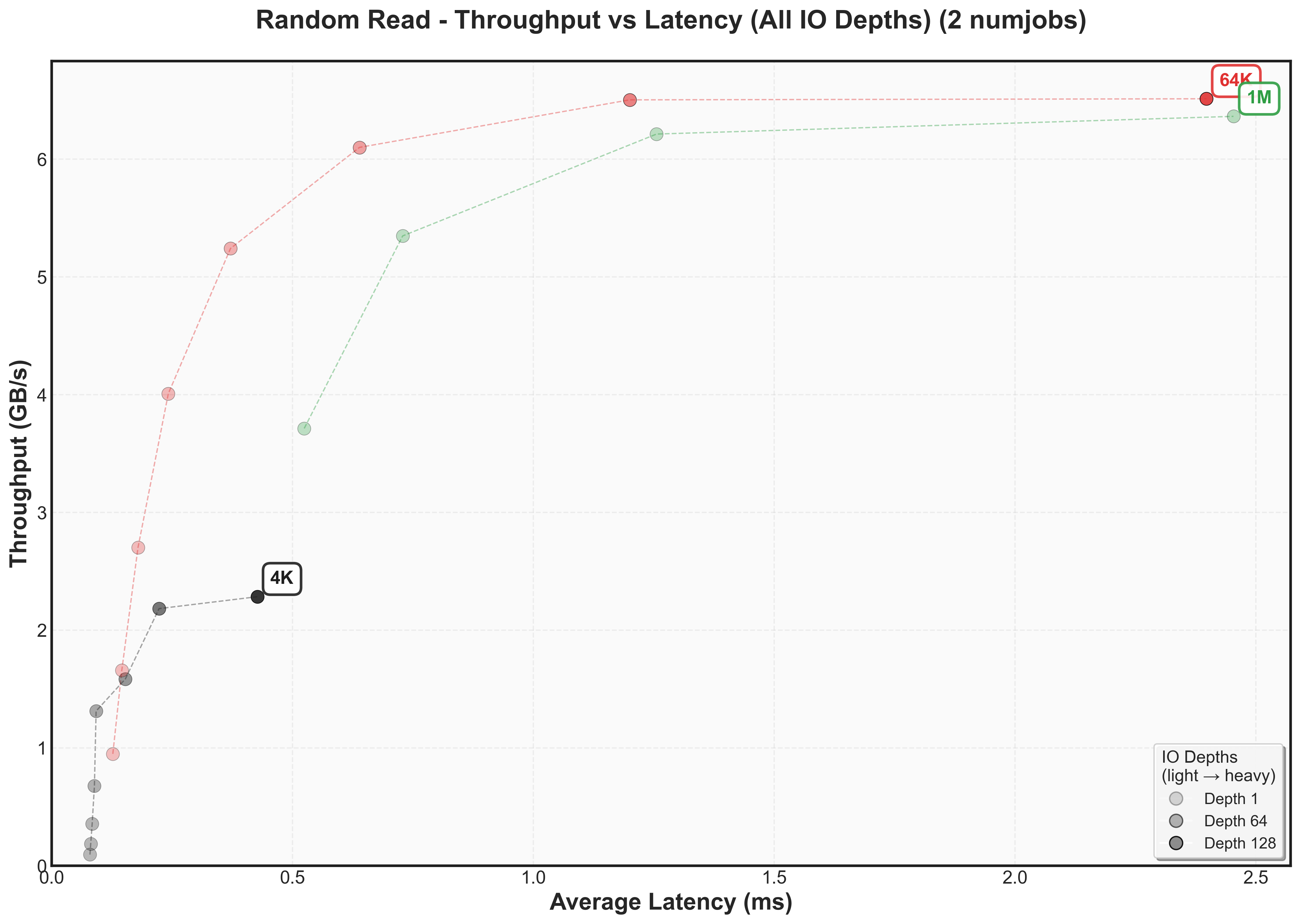
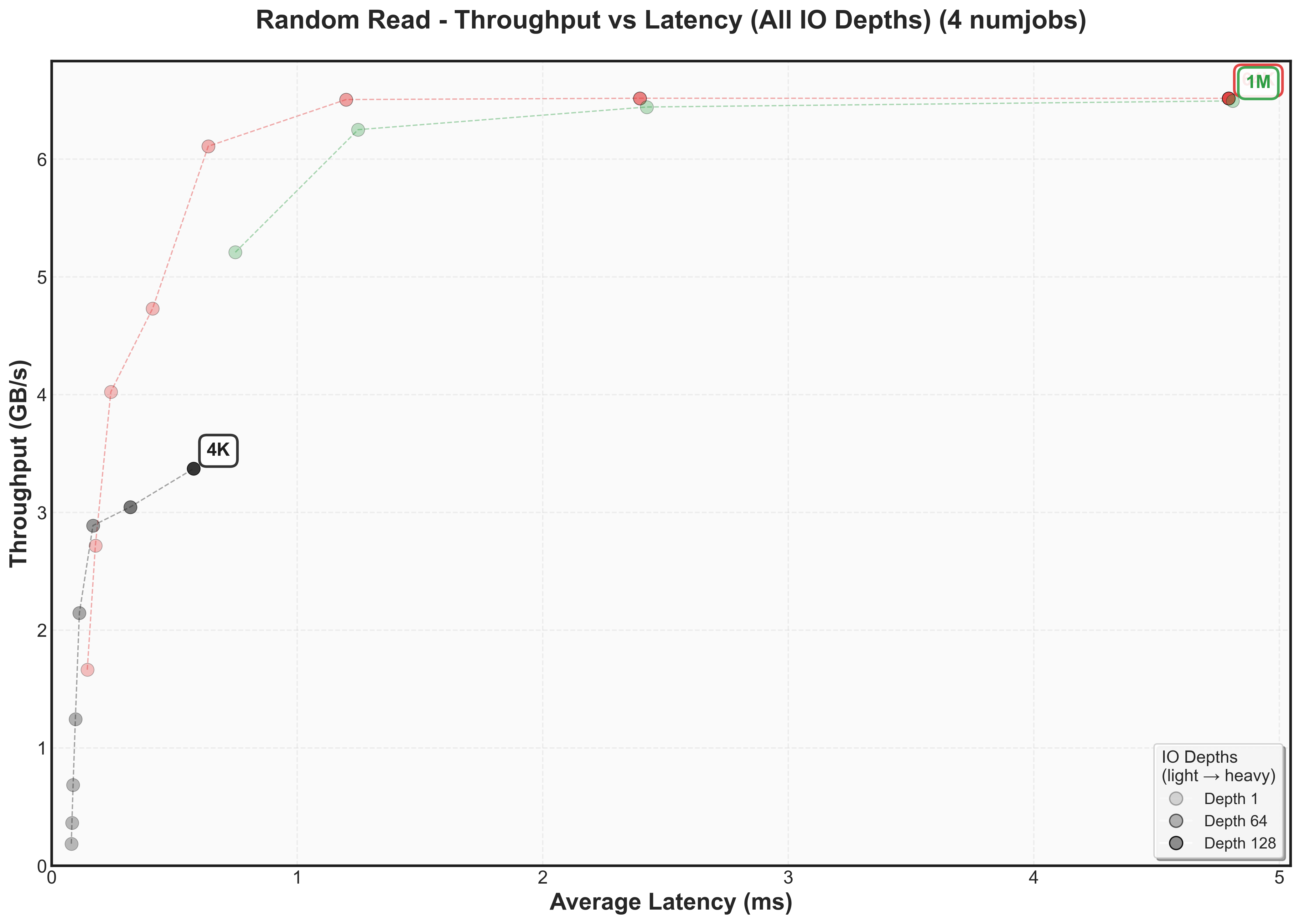
Storage Performance Analysis for local NVMe
Let’s examine how the NVMe drive performs compared to our SATA baseline:
Expand to view SATA SSD comparison graph
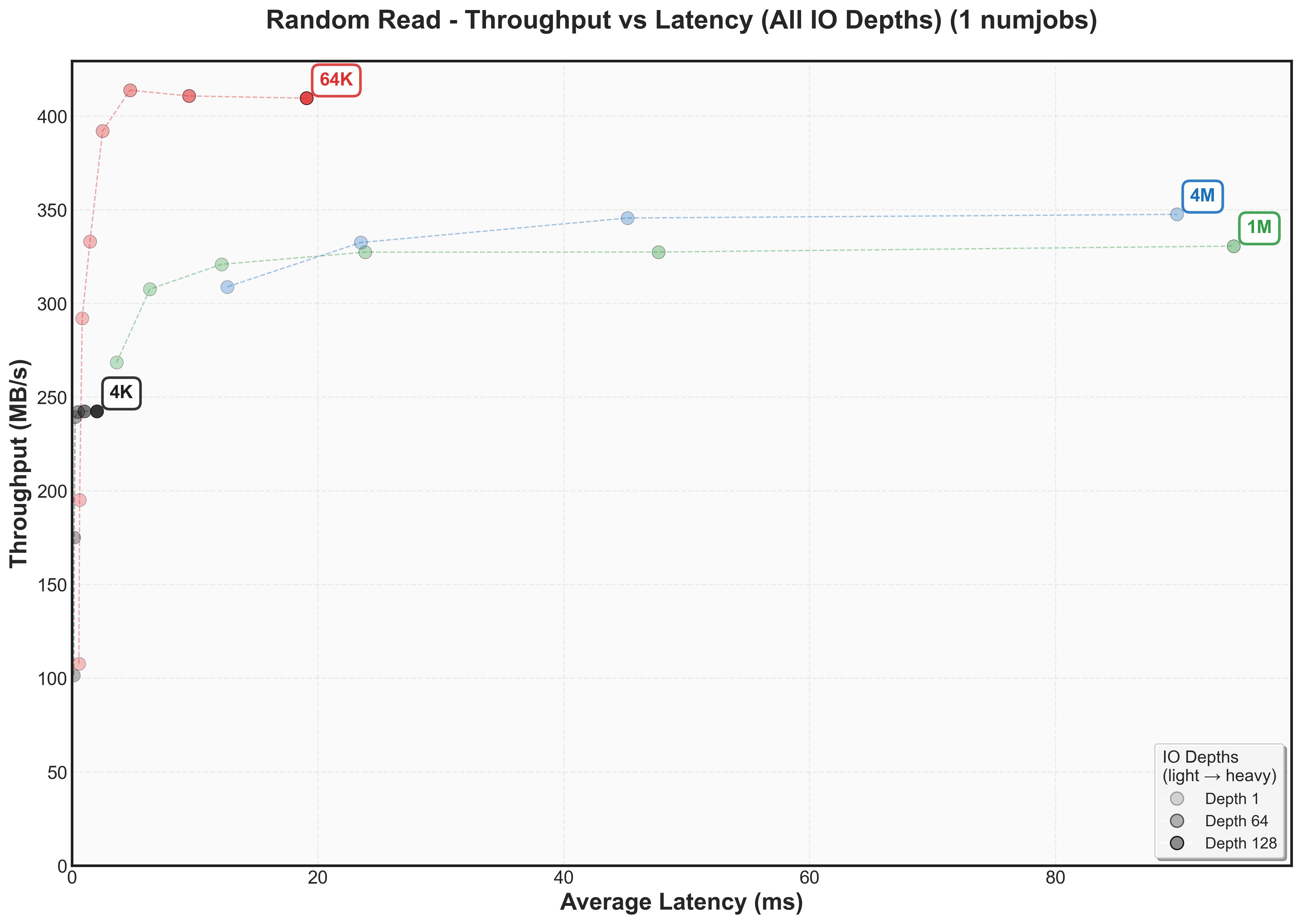
The NVMe improvement is dramatic:
- Throughput: 10x higher across all block sizes (1 GB/s vs 250 MB/s for 4K, 4 GB/s vs 400 MB/s for 64K)
- Latency: Consistently lower, especially for large blocksFor 64K blocks: NVMe stays at ~1ms while SATA climbs to ~20ms - a 20x difference
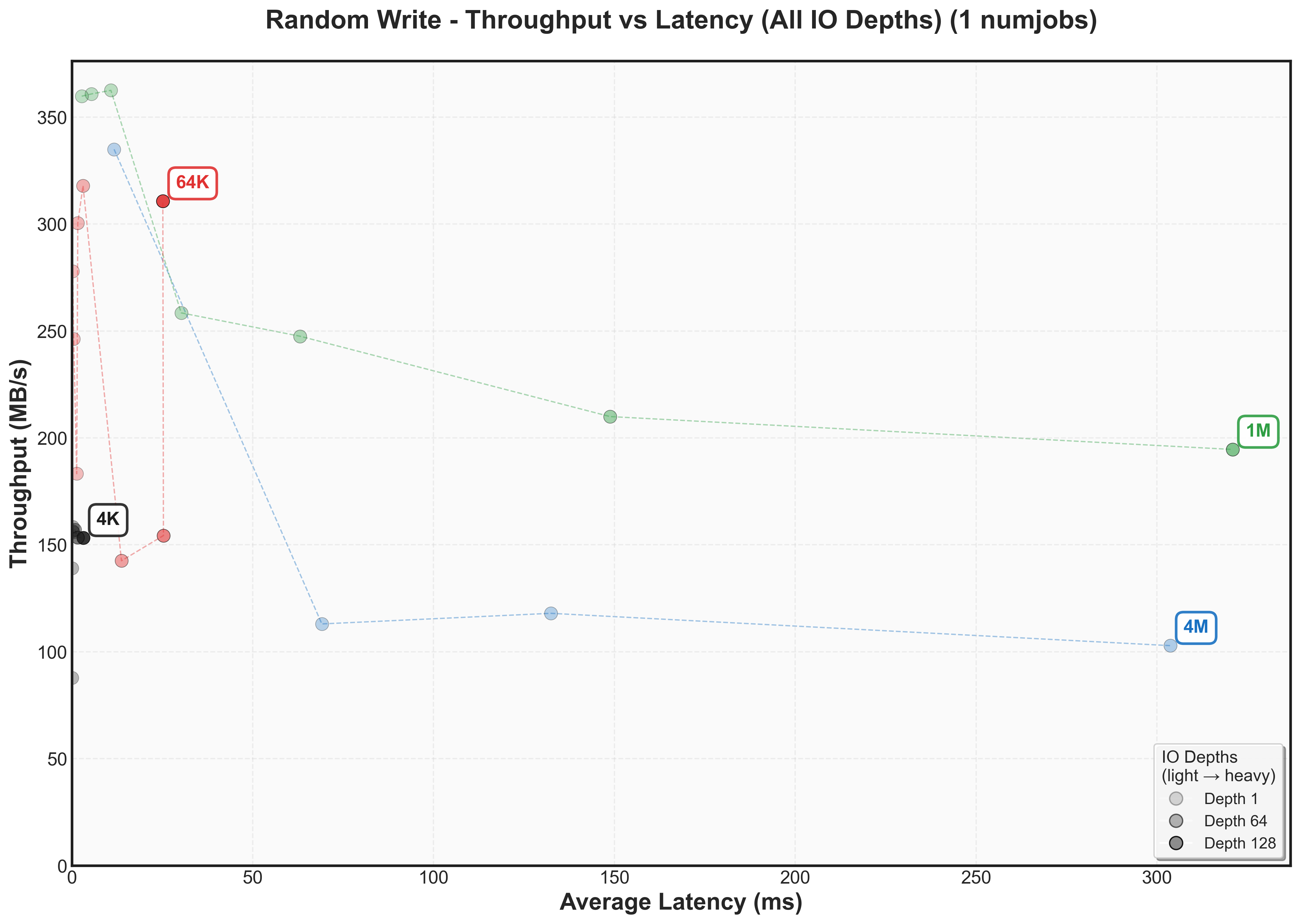
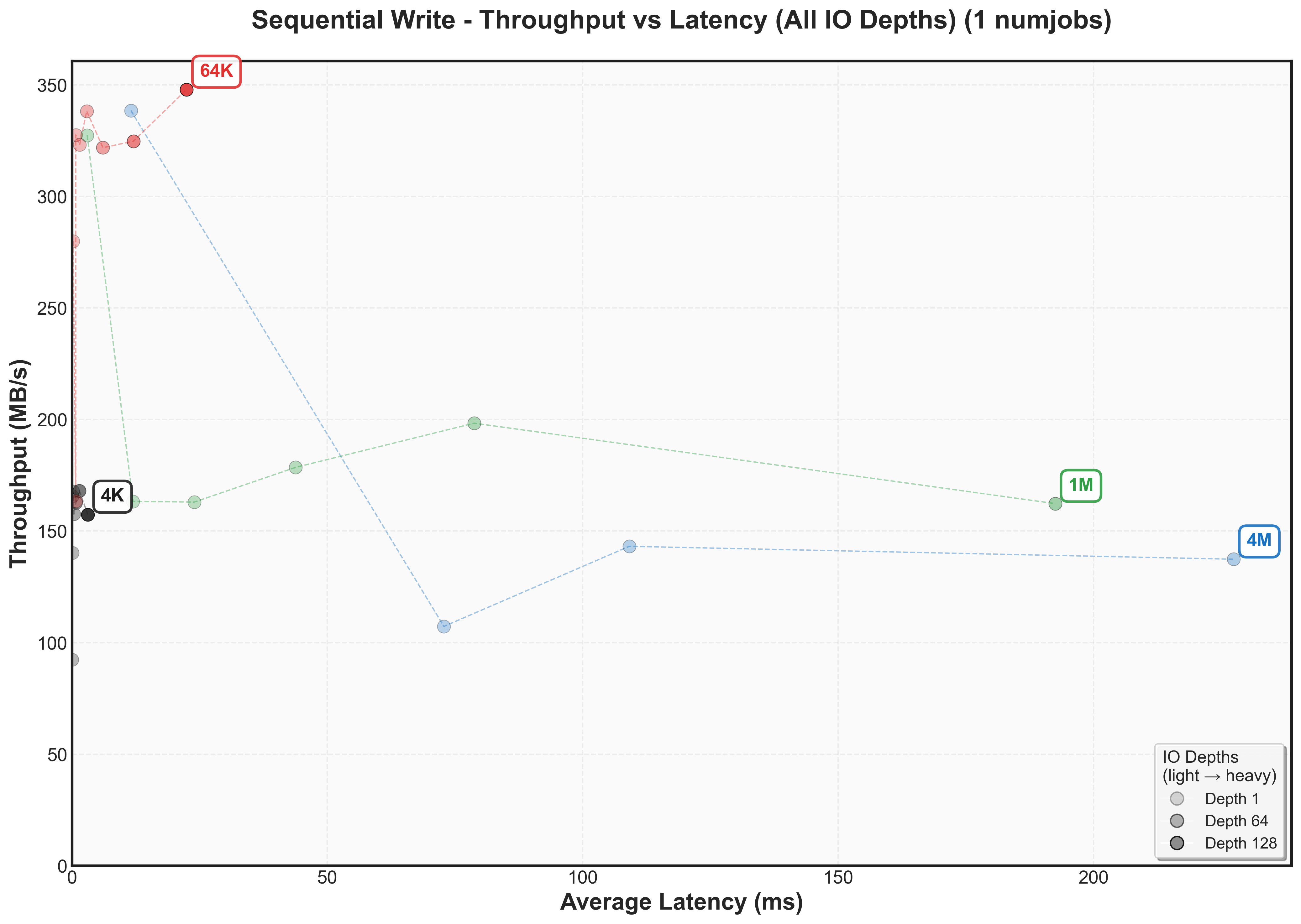
Two interesting differences from SATA patterns:
- 64K and 1M blocks need higher IO depths to hit their knee points, suggesting NVMe controllers require more parallelism for peak performance3FS may need to be configured with sufficient parallelism to extract maximum NVMe performance
Expand to view throughput versus latency graphs for other workloads

Expand to view throughput versus latency graphs scaling num jobs for random reads
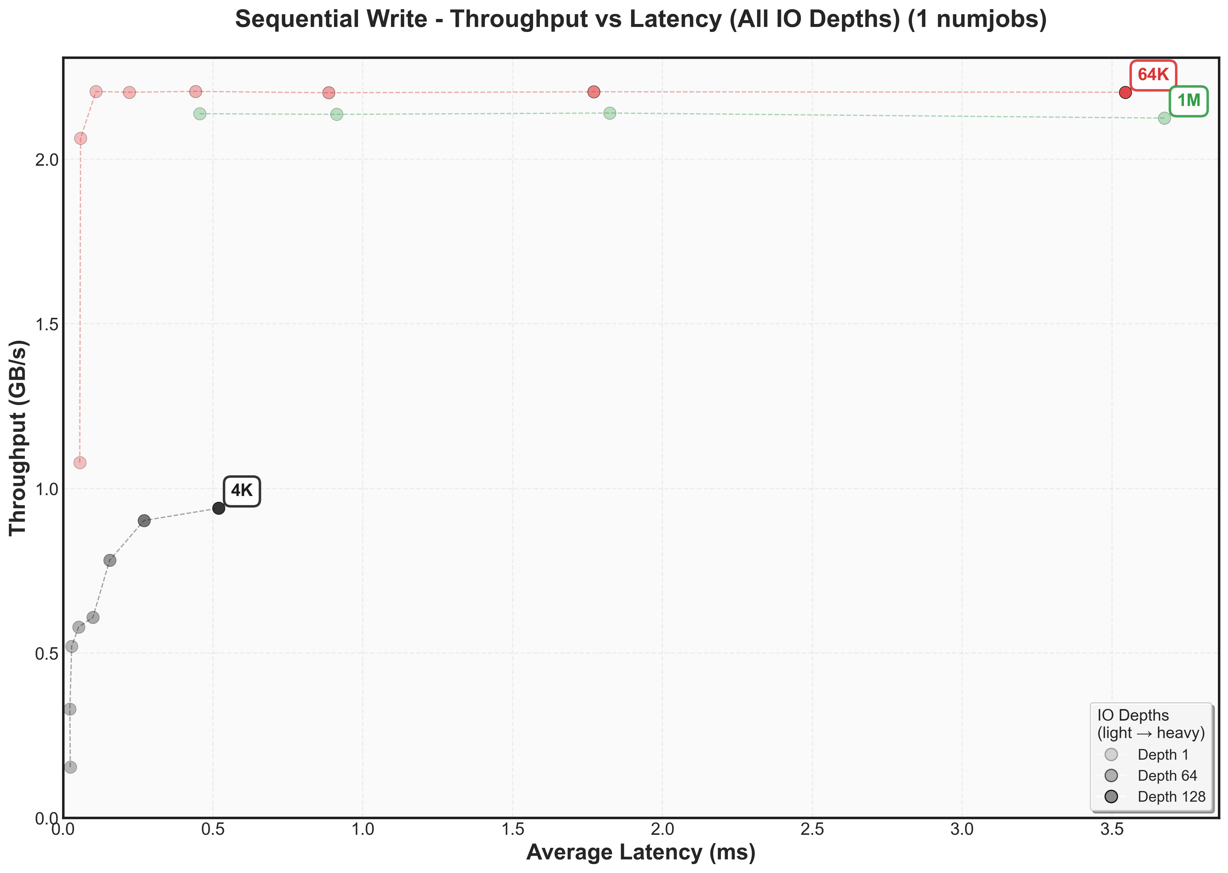
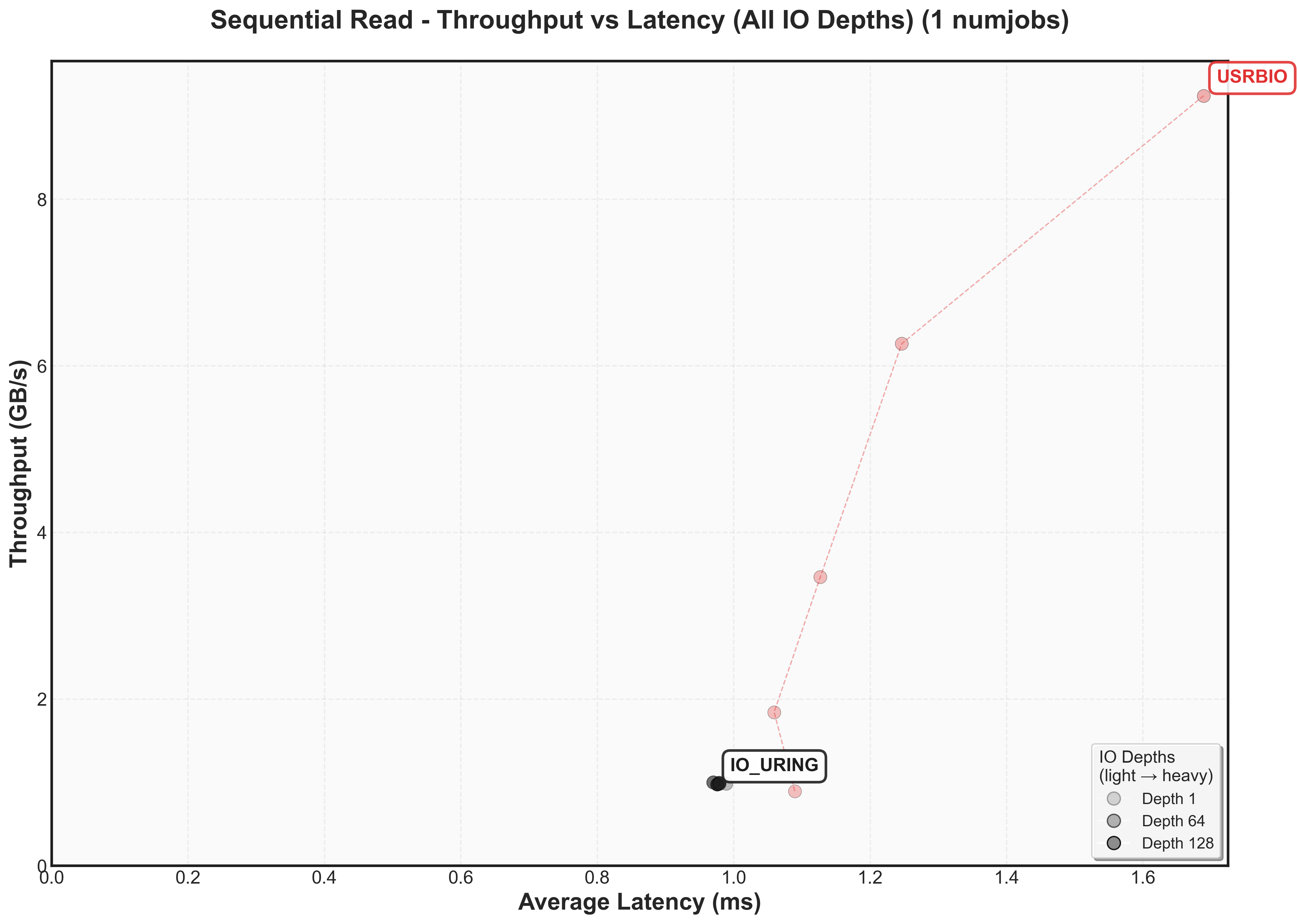
Sequential reads follow similar patterns to random reads, maintaining a similar high throughput ceiling and low latency.
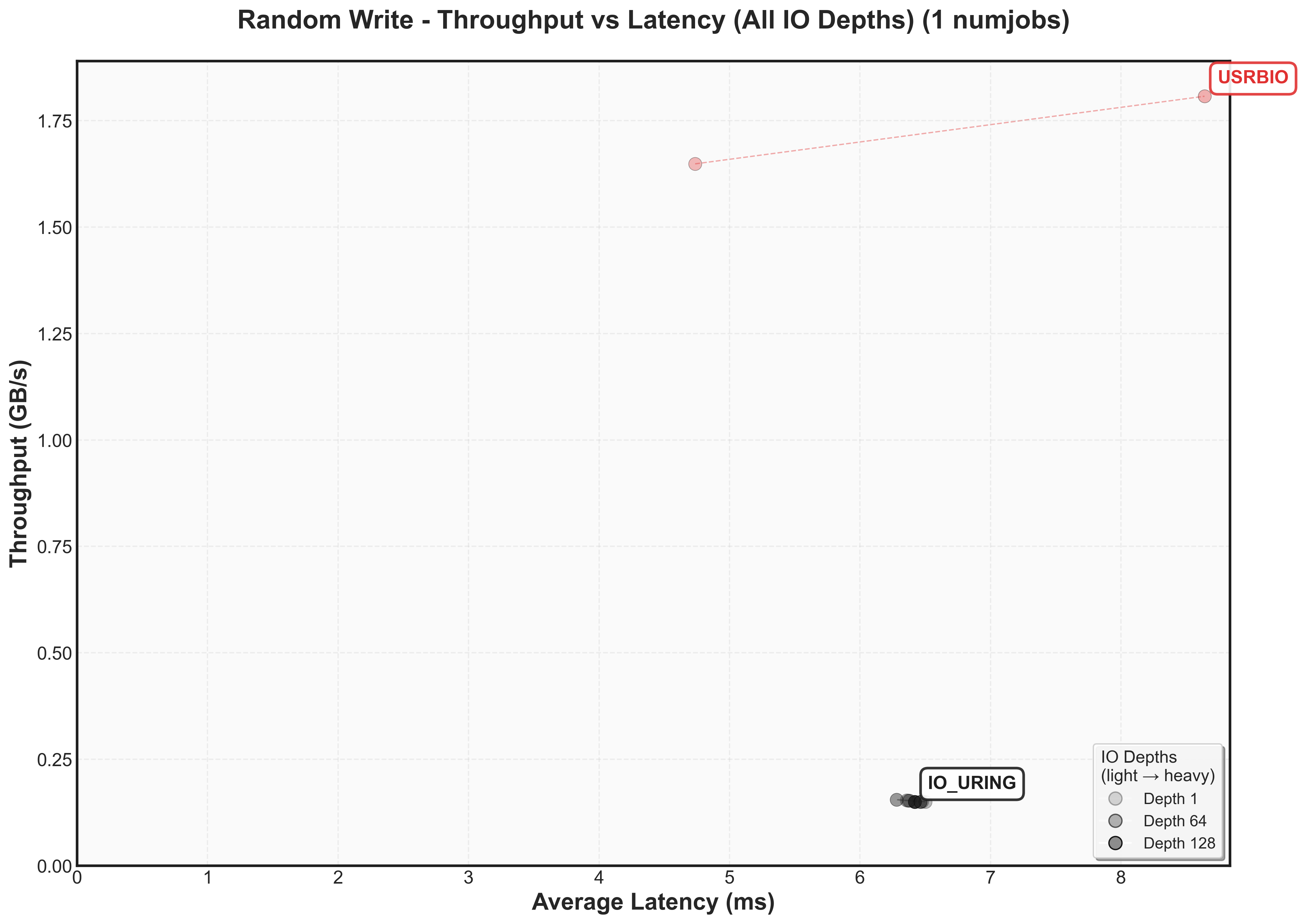
Write performance reveals a different story. Both random and sequential writes drop to ~2 GB/s peak throughput, with knee points occurring at much lower IO depths for 64K and 1M blocksThis aligns with the vendor specification showing NVMe write performance (2.3 GB/s) is significantly lower than read performance (6.2 GB/s).
The numjobs scaling patterns mirror what we observed with SATA SSDs: throughput increases with additional parallel jobs, but latency scales proportionally. Doubling jobs roughly doubles latency but provides less than 2x throughput improvement.
Predicting 3FS Performance
Before diving into actual 3FS benchmarks, let’s make some predictions based on our hardware baseline measurements:
For random/sequentials reads, our theoretical ceiling is 18 GB/s as there’s a replication factor of 3 and both random/sequential reads hit 6 GB/s.
However, we’re bound by network bandwidth as it as a theoretical limit of 12.5 GB/s (realistically ~11.5 GB/s from our previous micro-benchmarks).
Let’s now talk about latency in the worst and best case. We can pull the network and disk latency from the graphs we have, starting with reads.
In the average case:
- The average network latency for 1MB of data is 91us
- The average disk latency for sequential/random reads for 1M block size (1 IO depth, 1 job) is 0.48ms
- So the the latency we should expect is 0.48ms
In the worse case:
- The p99 network latency for 1MB of data is 282us
- The p99 disk latency for sequential/random reads for 1M block size (128 IO depth, 16 job) is 448ms/420ms
- So the the latency we should expect is 448ms
What we can see is a 100x difference in latency between the average and worse case. Another thing that we can clearly see that the latency is dominated by disk latency.
Moving on to writes,
Average case:
- 91us
- 0.46ms (1 IO depth, 1 job)
- So, latency combined is 0.46ms * 3 (chained) = 1.38ms
P99 case:
- 187us
- 892ms (128 IO depth, 16 job)
- So, latency combined is 892ms * 3 (chained) = 2.67s
Writes can be 2000x+ slower in the worse case. This is due to the multiplicative factor of writes since writes have to go through each node.
Keeping in this mind, let’s head into the benchmarks:
3FS
3FS is benchmarked using two different I/O interfaces: io_uring, the standard Linux asynchronous I/O interface, or USRBIO, a custom FIO engine that integrates directly with 3FS’s I/O queue management system.
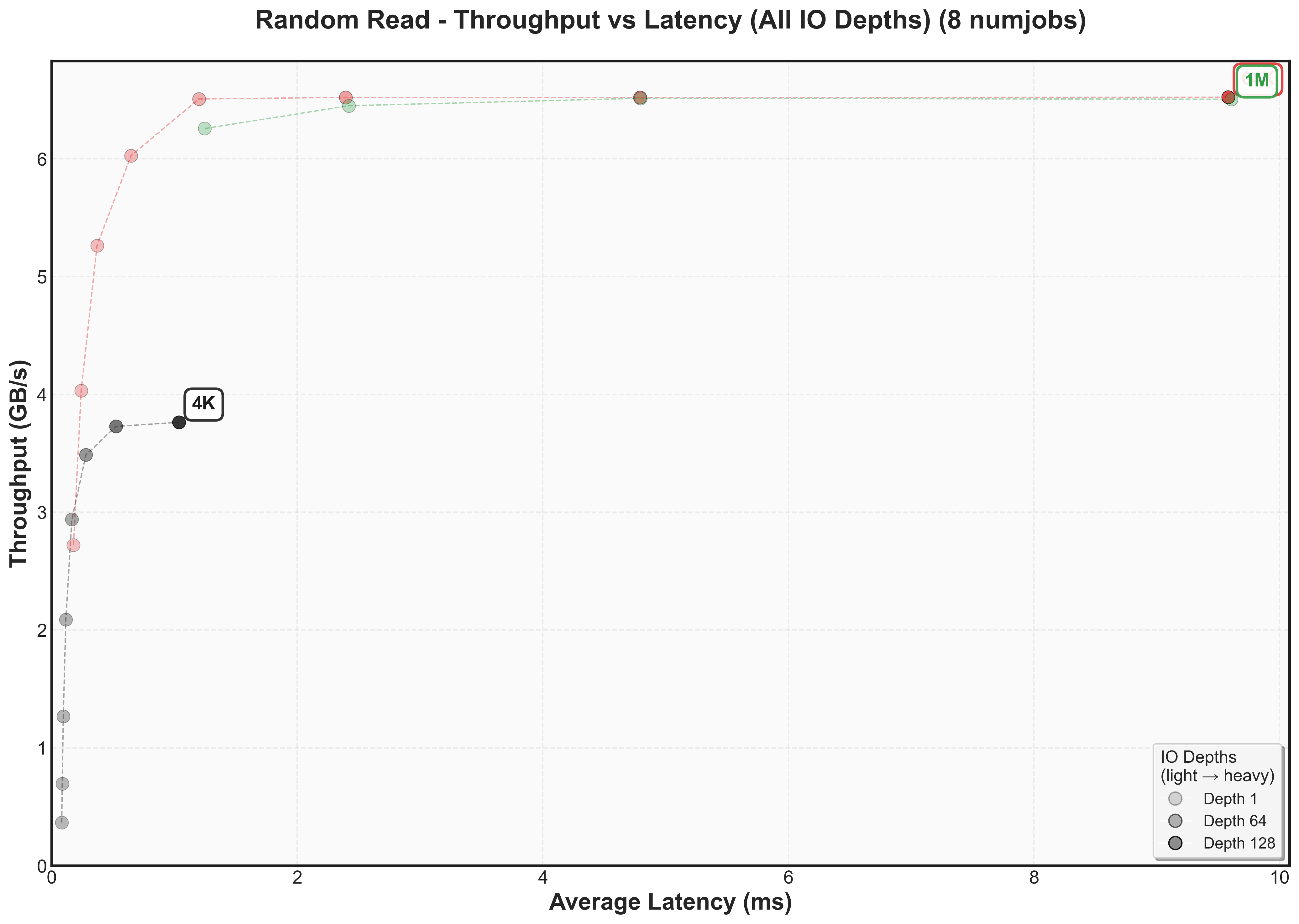
IO_URING
1M Block Size - HF3FS XFS with IO_URING (Modern)
Latency Percentiles
Performance of HF3FS with XFS filesystem using IO_URING driver on modern cluster with 1M block size.
USRBIO
1M Block Size - HF3FS XFS with USRBIO (Modern)
Latency Percentiles
Performance of HF3FS with XFS filesystem using USRBIO driver on modern cluster with 1M block size.
One thing to observe is that for io_uring, io_depth does not affect the performance.
Again, here’s the 2D graph. Do note that IO_URING is that same spot.
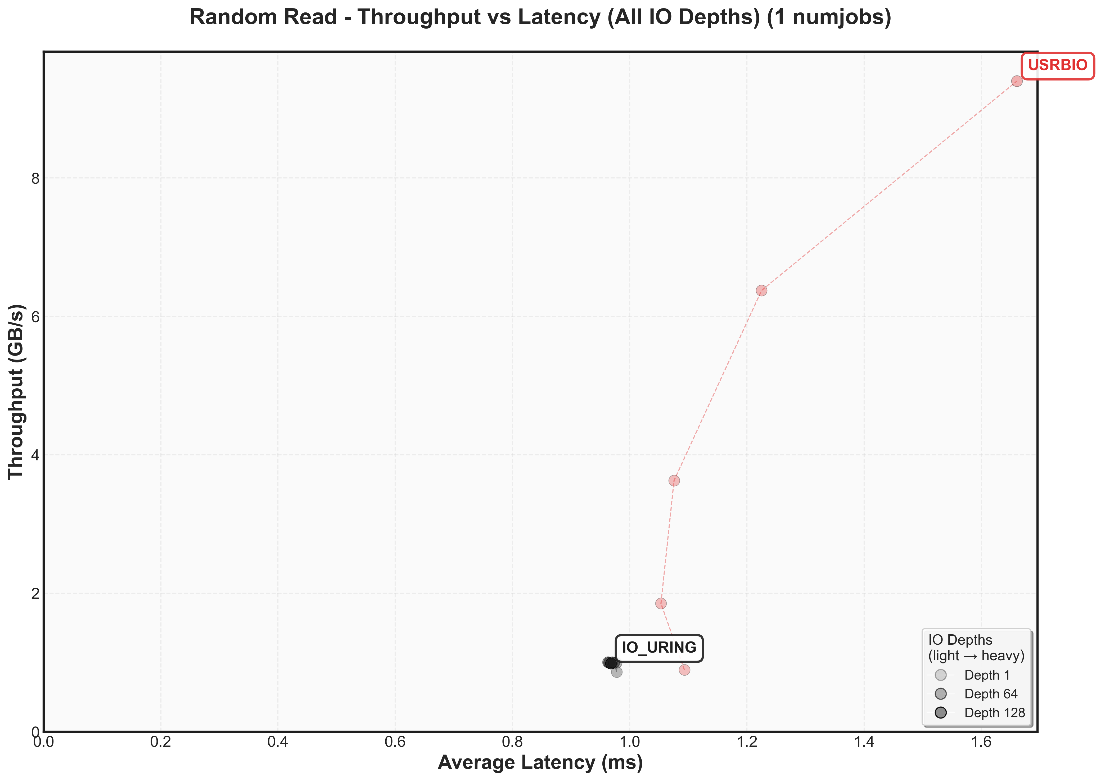
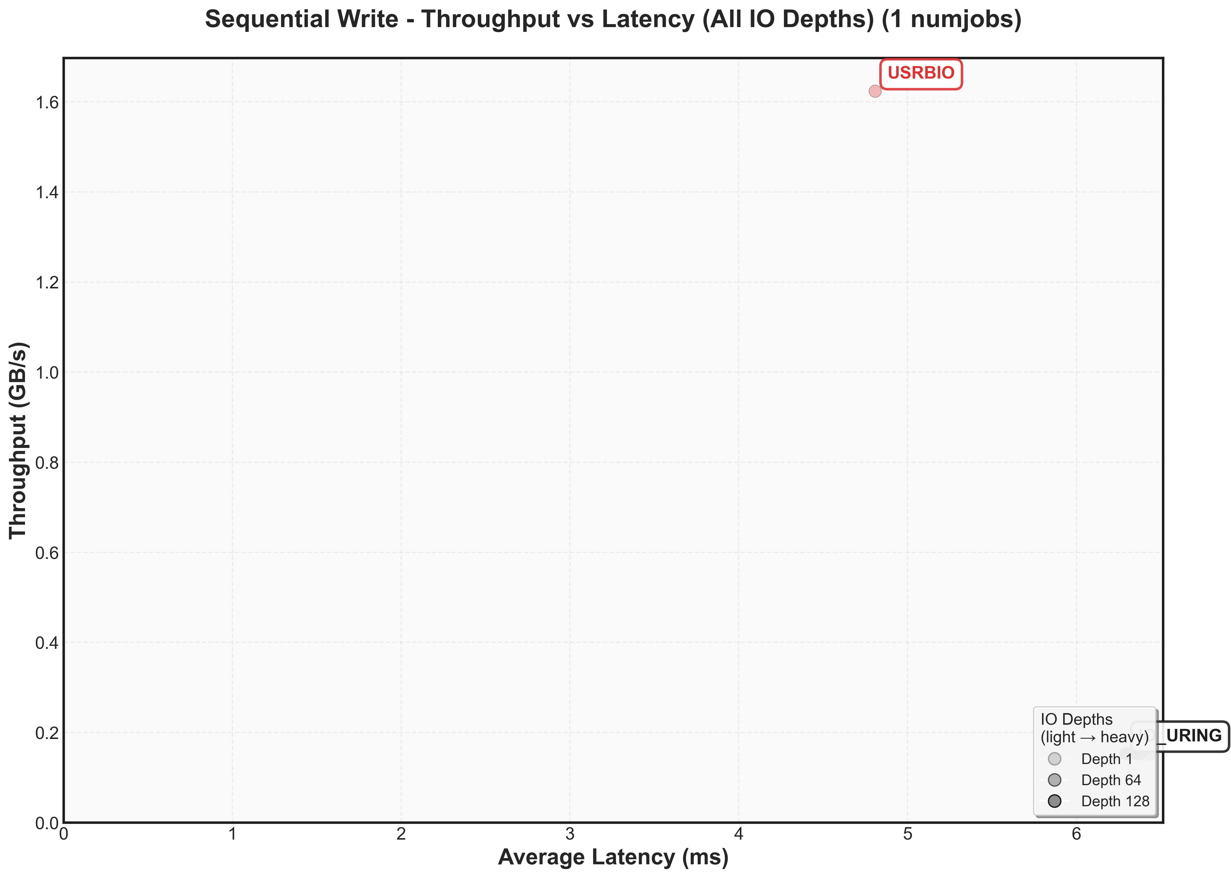
One interesting thing to observe is that io_uring has lower latency at the same throughput as usrbio.
Expand to view throughput versus latency graphs for other workloads
Does the performance match the estimates?
| Metric | Predicted | Actual |
|---|---|---|
| Read Latency (1MB) | 0.48ms | 1.09ms (127% worse) |
| Read P99 Latency | 304ms | 194ms (36% better) |
| Read Bandwidth | 11.5 GB/s | 10.3 GB/s (10% worse) |
| Write Latency (1MB) | 1.38ms | 2.55ms (85% worse) |
| Write P99 Latency | 0.89s | 1.1s (24% worse) |
| Write Bandwidth | 2.1 GB/s | 1.8 GB/s (14% worse) |
The 2x latency overhead for reads and writes may be coming from the software side of thingsWe’ll have to dig deeper later to see why. One interesting thing to see is that P99.9 latency is better for reads because the network bandwidth caps throughput before storage hits worst-case scenarios. What’s nice to see is that the bandiwdth only decreases by 10-15%!
3FS
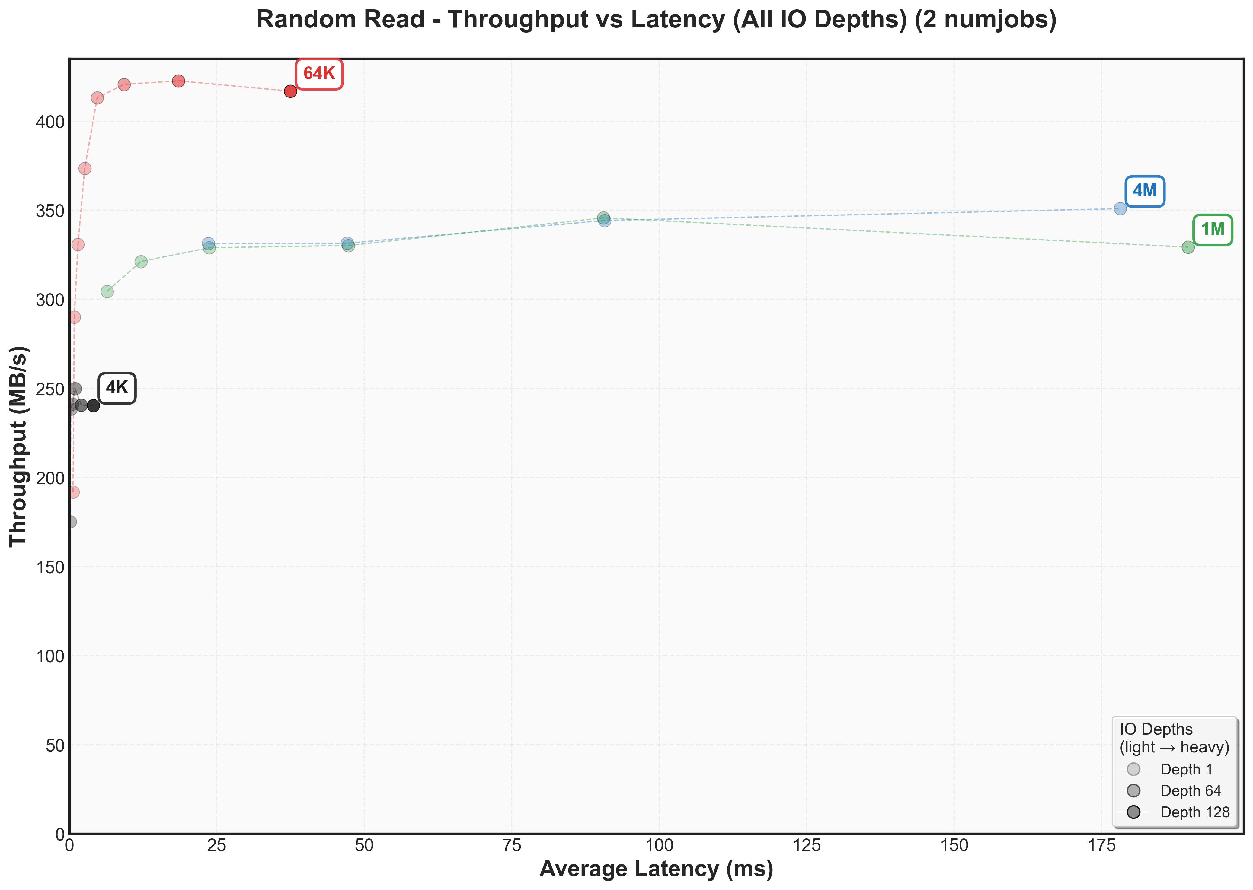
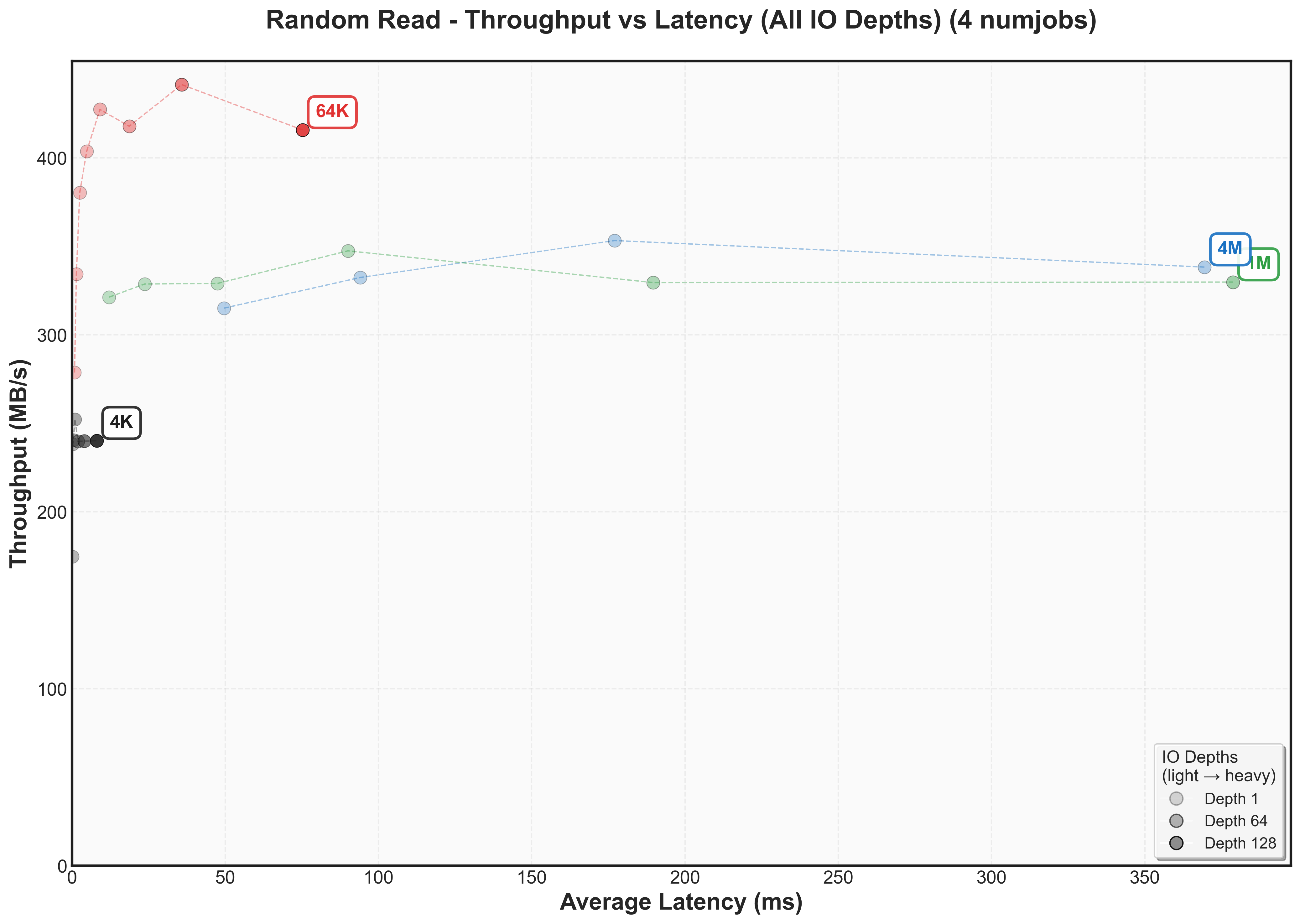
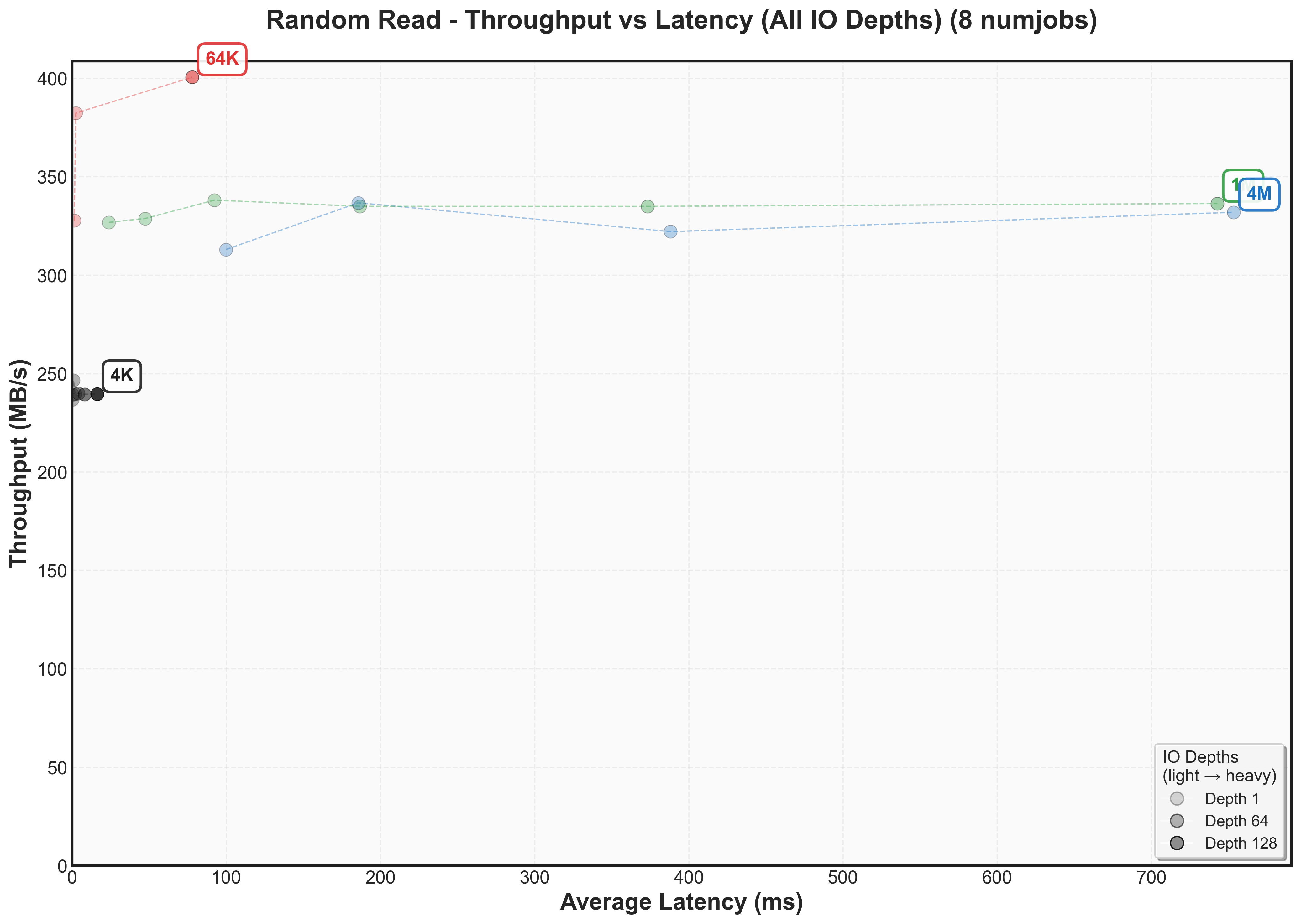
Now we examine how 3FS scales with block size and node count on the older cluster (SATA SSDs + 25 Gbps networking).
Scaling block size (5 nodes)
4K Block Size - HF3FS XFS with USRBIO (Older-5-Nodes)
Latency Percentiles
Performance of HF3FS with XFS filesystem using USRBIO driver with 4K block size on older cluster.
1M Block Size - HF3FS XFS with USRBIO (Older-5-Nodes)
Latency Percentiles
Medium block (1M) performance using HF3FS with XFS filesystem and USRBIO driver on older cluster.
The 4K block size stays well below the 3.25 GB/s network limit, reaching only 1 GB/s with 4ms latency. The 1M block size hits the network bandwidth ceiling but pays a latency penalty (6ms at 1 IO depth with 8 jobs compared to 4K’s 4ms maximum)
Scaling nodes
1M Block Size - HF3FS XFS with USRBIO (Older-5-Nodes)
Latency Percentiles
Medium block (1M) performance using HF3FS with XFS filesystem and USRBIO driver on older cluster.
1M Block Size - HF3FS XFS with IO_URING (Older-18-Nodes)
Latency Percentiles
Performance of HF3FS with XFS filesystem using IO_URING driver with 1M blocks on 18 node configuration.
Comparing 5 vs 18 nodes with 1M blocks shows latency increases with cluster size. At 18 nodes, scaling jobs works better than scaling IO depth for latency: 8 jobs/1 IO depth achieves 10ms @ 1.25 GB/s while 1 job/128 IO depth hits 90ms @ 1 GB/s.
With 18 nodes at 300 MB/s each, we’d expect 5.4 GB/s total, but the 25 Gbps network caps us at 3.25 GB/s and realistically we get 2.35 GB/s.
One thing that is a glaring issue are that after a certain point, the throughput drops rather significantly. The local results hold the bandiwidth. I’m not entirely sure now why that is, but configuration seems to me even more important as the throughput can decrease drasitcally.
Watch out for really large block sizes
4M Block Size - HF3FS XFS with USRBIO (Older-18)
Latency Percentiles
Large block (4M) performance using HF3FS with XFS filesystem and USRBIO driver on 18 node configuration.
For 4M blocks, 3FS achieves 2.5 GB/s with just 1 IO depth and 8 jobsThis approaches 77% of the theoretical 3.25 GB/s network limit.. As you can see, increasing the number of nodes or the block sizes shifts the graph a little bit.
Wrapping up
The microbenchmarks reveal concrete performance characteristics for 3FS across different hardware configurations. We now have baseline numbers showing how 3FS compares to local storage and where the bottlenecks emerge.
- 3FS adds predictable overhead: ~1ms for reads, ~1.2ms for writes
- Network bandwidth becomes the limiting factor before storage saturation
- Performance scales reasonably with both block size and node count
The next step is testing 3FS with actual workloads to see how much the performance translates to practice. Since 3FS has a relatively generic interface, we can compare with many other systems.
Citation
To cite this article:
@article{zhu20253fs3,
  title = {Network Storage and Scaling Characteristics of a Distributed Filesystem},
  author = {Zhu, Henry},
  journal = {maknee.github.io},
  year = {2025},
  month = {September},
  url = "https://maknee.github.io/blog/2025/3FS-Performance-Journal-3/"
}
Enjoy Reading This Article?
Here are some more articles you might like to read next: